Troyan V., Kiselev Y. Statistical Methods of Geophysical Data Processing
Подождите немного. Документ загружается.


Statistical criteria for choice of model 213
In the formula (7.21) the terms in the second square brackets do not depend on
θ
θ
θ
m
. From the above formula we can conclude that if all signals
f
f
µk
are known,
except only one signal θ
θ
θ
m
, then for the determination of θ
θ
θ
m
we can maximize the
expression in the first square brackets of the formula (7.21). This expression we
denote as g
m
(u
k
, θ
m
) and write down in the form
g
m
(
u
u
k
,
θ
θ
m
) =
X
k
Y
Y
T
km
R
−1
f
f
mk
(
θ
θ
m
) −
1
2
X
k
f
f
f
T
mk
(
θ
θ
m
)R
−1
f
f
mk
(
θ
θ
m
), (7.22)
where
Y
T
km
=
u
u
T
k
−
M
X
µ=1
µ6=m
f
f
T
kµ
(θ
µ
). (7.23)
The expression g
m
(
u
u
k
,θθ
m
) makes a sense of the sufficient reception function for
a single signal with a number m, but there instead of the measured data u
k
the
model data Y
mk
is used. The model data is obtained by the subtraction from the
measured data of the signals
f
f
µk
with indices µ 6= m.
The idea of the iterative process consists in reiterated and by turn look-up of
the vectors
θ
θ (m = 1, 2, . . . , M) with the help of the sufficient reception function
(7.22) and with the use of the values of others parameters which were found in the
previous iterations of θ
µ
(µ 6= m). If we do not know the number of signals M, then
the computing circuit looks as following.
At the beginning it is assumed that we have only one signal and we determine
its parameters by minimizing of the sufficient reception function (7.22) at m = 1:
g
1
(uu
k
,θθ
1
) =
X
k
uu
T
k
R
−1
f
k
(θ
1
) −
1
2
f
T
k
(θ
1
)R
−1
f
k
(θθ
1
)
. (7.24)
We find a maximum of the function g
m
(uu
k
,θθ
1
), using, for example, one of the
gradient methods:
ˆ
θ
(1)
1
= max
θ
θ
1
g
1
(u
k
, θ
1
).
Then, we suppose that there are two signals and we find the second vector
ˆ
θθ
(1)
2
by
maximizing of
g
2
(
u
u
k
,
ˆ
θθ
1
,θθ
2
) =
X
k
Y
T
k2
R
−1
f
f
k2
(θ
2
) −
1
2
X
k
ff
T
k2
(θ
2
)R
−1
f
k2
(θθ
2
),
where
Y
Y
T
k2
= uu
T
k
− f
k1
(
ˆ
θθ
1
).
After that, taking into account that we have two signals, we again find the vector
ˆ
θθ
(1)
1
by maximizing of
g
2
(
u
u
k
,
θ
θ
1
,
ˆ
θ
θ
(1)
2
) =
X
k
Y
Y
T
k1
R
−1
f
f
f
k1
(
θ
θ
1
) −
1
2
X
k
f
f
f
T
k1
(
θ
θ
1
)R
−1
f
f
k1
(θ
θ
θ
1
),
Y
k1
= u
T
k
−ff
k2
(
ˆ
θ
2
),

214 STATISTICAL METHODS OF GEOPHYSICAL DATA PROCESSING
at that we use the obtained estimates
ˆ
θ
(1)
2
. Then we find
ˆ
θθ
(2)
2
, supposing that
ˆ
θθ
(1)
1
is equal to the obtained values, etc. The values of the maxima of the sufficient
reception function, obtained in the process of the parameters refinement, are an
increasing number sequence. We stop the procedure if the values of the maxima
become stable.
If
g
2
(
ˆ
θ
(n)
1
,
ˆ
θ
θ
(n)
2
) − g
2
(
ˆ
θ
θ
(n−1)
1
,
ˆ
θ
(n−1)
2
)
g
2
(
ˆ
θθ
(n−1)
1
,
ˆ
θ
(n−1)
2
)
< δ,
then the refinement can be stopped at δ ∼ 10
−2
÷ 10
−3
. Further, we suppose that
we have three signals and we find the vector
ˆ
θ
θ
(1)
3
by maximizing
g
3
(
u
u
k
,
ˆ
θ
θ
1
,
ˆ
θ
θ
θ
2
,θ
θ
θ
3
) =
X
k
Y
Y
T
k3
R
−1
f
f
f
k3
(
θ
θ
3
) −
1
2
X
k
f
f
f
T
k3
(
θ
θ
3
)R
−1
f
f
k3
(θ
θ
θ
3
),
YY
T
k3
= u
T
k
−
f
f
T
k1
(
ˆ
θ
1
) −ff
T
k2
(
ˆ
θ
2
),
where
ˆ
θ
θ
1
,
ˆ
θ
θ
2
are the estimates obtained after refinement. Then we find again of
ˆ
θ
θ
θ
1
, with fixing of
ˆ
θ
θ
θ
2
and
ˆ
θ
θ
θ
3
by obtained values. After that we find θ
θ
θ
(1)
2
under fixed
values of
ˆ
θ
θ
(1)
1
and
ˆ
θ
θ
θ
(1)
3
, and etc. During the implementation of such calculations we
suppose that we have three signals and we make the cyclic rearrangement of the
indices µ. We stop the refinement if an increment of the value of the maximum
becomes small enough:
g
3
(
ˆ
θ
θ
(n)
1
,
ˆ
θ
(n)
2
,
ˆ
θ
(n)
3
) − g
3
(
ˆ
θ
θ
(n−1)
1
,
ˆ
θ
(n−1)
2
,
ˆ
θ
θ
(n−1)
3
)
g
3
(
ˆ
θ
θ
θ
(n−1)
1
,
ˆ
θ
θ
(n−1)
2
,
ˆ
θ
θ
θ
(n−1)
3
)
< δ.
Further we suppose that there are four signals and again we refine the parameters of
the signals
θ
θ
m
by the cyclic rearrangement of the indices µ = 1, 2, 3, 4. In each step
we maximize the sufficient reception function (7.22) with the use of the appropriate
modified data (7.23). Each time at the determination of the signal parameters for
new value of M = m, the threshold condition is tested
α
m
≥ α
0
,
where α
m
corresponds to the extraction of the single regular wave with the given
probability of the error (7.7):
P
e
= Φ(−α
m
/2), α
m
=
"
X
k
f
T
mk
(
ˆ
θθ
m
)R
−1
f
f
mk
(
ˆ
θ
m
)
#
1/2
.
In the special case of the uncorrelated random component R = σ
2
I with the prob-
ability of the error of 0.05 the threshold condition for the seismic signal
f
f
k
(θ
m
) = kA
m
ϕ(t
i
− τ
m
− k∆xγ
m
)k
n
i=1

Statistical criteria for choice of model 215
has the form
A
m
σ
"
X
k
ϕ
2
(t
i
− τ
m
− k∆xγ
m
)
#
1/2
≥ α
m
= 3.3,
at that, the value of α
m
is the signal-to-noise ratio. The sufficient reception function
(7.22) for a seismic signal at given assumptions reads as
g(A
m
, τ
m
, γ
m
) =
A
m
σ
2
X
i
ϕ(t
i
)
X
k
y(t
i
+ τ
mk
) −
A
2
m
σ
2
K
X
i
ϕ
2
(t
i
), (7.25)
y(t
i
+ τ
mk
) = u(t
i
+ τ
mk
) −
X
µ
0
6=m
A
µ
0
ϕ(t
i
− τ
µ
0
k
− τ
µk
). (7.26)
Maximizing the function (7.25) over the amplitude A
m
, we obtain the estimate in
the explicit form
ˆ
A
m
=
P
i
ϕ(t
i
)
P
k
y(t
i
+ τ
mk
)
P
i
ϕ
2
(t
i
)
. (7.27)
Substituting the formula (7.27) to the expression (7.25) we obtain the function
which depends on kinematic parameters only
g
m
(τ
m
, γ
m
) =
1
σ
2
P
i
ϕ(t
i
)
P
k
y(t
i
+ τ
mk
)
2
K
P
i
ϕ
2
(t
i
)
. (7.28)
After analysis of the formula (7.28) we can conclude that the sufficient re-
ception function in the parameter space (the arrival time and the apparent slow-
ness) corresponds to a summogram of the controlled directional reception (CDR)
P
k
Y (t
i
+ τ
mk
) with the subsequent optimum filter. Let us note, that CDR sum-
mogram is the discrete analog of the Radon transform in a seismogram plane.
This page intentionally left blankThis page intentionally left blank
Chapter 8
Algorithms of approximation of
geophysical data
In areas with a compound subsurface geology at the constructing of the model of
a geophysical field and at the solution of the inverse geophysical problems the ap-
proximation and interpolation of geophysical data by the spline functions and a
piecewise-polynomial approximation are widely used (Ahlberg et al., 1967; Schu-
maker, 2007; Aronov, 1990; Sudvarg, 1974). Such approach enables to describe the
geophysical fields of the various smoothness, that is typical for geophysical data
(Volkov, 1981; Troyan, 1981b). We shall consider univariate cubic splines, paramet-
ric splines, splines of the fourth order together with the examples of their application
for the processing of geophysical data.
For the case of an areal spread, the problem of imaging of a spatial seismic
section subject to borehole data is actual. We shall consider an example of the
seismic horizon imaging with the use of an areal spread and borehole data.
8.1 The Algorithm of Univariate Approximation by Cubic Splines
Let’s on the abscissa axis in the points
x
1
< x
2
< ··· < x
K
(8.1)
the values of the observed function are given
u
1
, u
2
, . . . , u
K
. (8.2)
Here we suppose a monotone increasing of the argument x that is easily satisfied in
the practice.
From the beginning we consider an application of the spline functions for the in-
terpolation problem (Schumaker, 2007). The interpolating cubic spline is a function
ϕ(x), which in the nodes x
k
is equal to
ϕ(x
k
) = u
k
, (8.3)
and inside the intervals (x
k
, x
k+1
) it is determined by the cubic polynomials f
k
(x),
which in the points x
k
(k = 2, 3, . . . , K −1) are supposed doubly differentiable:
f
k
(x) = a
k
(x − x
k
)
3
+ b
k
(x − x
k
)
2
+ c
k
(x − x
k
) + d
k
. (8.4)
217

218 STATISTICAL METHODS OF GEOPHYSICAL DATA PROCESSING
For the determination of such interpolation function we should find 4(k −1) of the
coefficients a
k
, b
k
, c
k
, d
k
.
Let us consider an arbitrary interval x
k
, x
k+1
. The spline function in the bound-
ary points of the interval x
k
and x
k+1
must satisfy to the next conditions
ϕ(x
k
) = f
k
(x
k
) = d
k
,
ϕ(x
k+1
) = f
k
(x
k+1
) = a
k
∆x
3
k
+ b
k
∆x
2
k
+ c
k
∆x
k
+ d
k
, (8.5)
ϕ
0
(x
k
) = f
0
k
(x
k
) = c
k
,
ϕ
0
(x
k+1
) = f
0
k
(x
k+1
) = 3a
k
∆x
2
k
+ 2b
k
∆x
k
+ c
k
, (8.6)
ϕ
00
(x
k
) = f
00
k
(x
k
) = 2b
k
,
ϕ
00
(x
k+1
) = f
00
k
(x
k+1
) = 6a
k
∆x
k
+ 2b
k
. (8.7)
The values of desired coefficients can be found using the conditions (8.5), (8.7) for
the first and the second derivatives, and relation (8.3). After the analytic transfor-
mation we obtain
a
k
=
1
6∆x
k
(ϕ
00
(x
k+1
) − ϕ
00
(x
k
)),
b
k
=
1
2
ϕ
00
(x
k
),
c
k
=
∆u
k
∆x
k
−
1
6
∆x
k
(ϕ
00
(x
k+1
) + ϕ
00
(x
k
)),
d
k
= u
k
, (8.8)
where ∆u
k
= u
k+1
−u
k
. Using the condition (8.6) and formulas for the coefficients
(8.8), we obtain the formulas for the first derivatives of the spline functions
ϕ
0
(x
k
) =
∆u
k
∆x
k
−
1
6
∆x
k
(ϕ
00
(x
k+1
) + 2ϕ
00
(x
k
)),
ϕ
0
(x
k
) =
∆u
k−1
∆x
k−1
−
1
6
∆x
k−1
(ϕ
00
(x
k
) + 2ϕ
00
(x
k−1
),
k = 1, 2, . . . , K − 1. For the determination of the second derivatives ϕ
00
(x
k
) of the
spline functions we require a continuity of the first derivative in the boundary of
two intervals
f
0
(x
k
) = f
0
k
(x
k
), k = 2, 3, . . . , K − 1. (8.9)
Substituting the condition (8.6) into the expression (8.9), we obtain
3a
k−1
∆x
2
k−1
+ 2b
k−1
∆
x
k − 1c
k−1
= c
k
.
Using the representation (8.8) for the coefficients, we obtain the system of equations
∆
k−1
ϕ
00
(x
k−1
) + 2(∆x
k−1
+ ∆x
k
)ϕ
00
(x
k
) + ∆x
k
ϕ
00
(x
k−1
)
= 6
∆u
k
∆x
k
−
∆u
k−1
∆x
k−1
. (8.10)

Algorithms of approximation of geophysical data 219
Using the system of K −2 equations (8.10) we can determine the unknown ϕ
00
(x
k
),
then, taking into account the values of u
k
, we find the coefficients a
k
, b
k
, c
k
, d
k
with the help of (8.8). Before calculation we must designate the values of ϕ
00
(x
1
)
and ϕ
00
(x
k
), which in the case of cubic spline usually are equal to zero:
ϕ
00
(x
1
) = ϕ
00
(x
k
) = 0. (8.11)
The formula (8.10) can be written down in a matrix form
Aϕ
00
= y, (8.12)
where
A =
2(∆x
1
+ ∆x
2
) . . . . . . 0
∆x
2
. . . . . . 0
. . . . . . . . . . . .
0 . . . ∆x
K−2
2(∆x
K−2
+ ∆x
K−1
)
.
The matrix A of the system (8.12) is a three-diagonal symmetric matrix with the
positive diagonal elements, consequently, it is a positive-defined matrix. Thus, an
unique existence of the solution of the system (8.12) is ensured. The solution can
be found, for example, by the Gauss elimination method (Voevodin and Kuznetsov,
1984).
Once it is more convenient to represent the conditions for the second derivative
in the form
ϕ
00
(x
1
) = αϕ
00
(x
2
), ϕ
00
(x
k−1
) = αϕ
00
(x
k
), (8.13)
where α, β are the arbitrary numbers. In the practice enough often to choose
α = β = 1, so far the second derivatives in the points x
1
and x
k
are equal to
the second derivatives in the points x
2
and x
k−1
respectively. Not infrequently the
equalities α = β = 1/2 are used.
Substituting the conditions (8.13) in the system of equations (8.10), and, for
k = 2 and k = K − 1, we obtain
((2 + α)∆x
1
+ 2∆x
2
)ϕ
00
(x
2
) + ∆x
2
ϕ
00
(x
3
) = 6
∆u
2
∆x
2
−
∆u
1
∆x
1
,
∆x
K−2
ϕ
00
(x
K−2
) + (2∆x
K−2
+ (2 + β)∆x
K−1
)ϕ
00
(x
K−1
)
= 6
∆u
K−1
∆x
K−1
−
∆u
K−2
∆x
K−2
.
Other equations remain without changing. This implies that in the matrix of the
system (8.12) only two elements in the first and last rows are varied. The first and
last components of the vector
y
y of absolute terms are varied also. In this case the
unique existence of the cubic splines is supplied by the conditions
−
∆x
2
∆x
1
+ 2
≤ α < ∞, −
∆x
K−2
∆x
K−1
+ 2
≤ β < ∞.

220 STATISTICAL METHODS OF GEOPHYSICAL DATA PROCESSING
Thus far we was considered the next scheme of the determination of the cubic
splines: for given x
k
, u
k
and for the boundary conditions (8.11) or (8.13) we de-
termine the vector of the second derivatives ϕ
00
by the solution of the system of
linear equations (8.12), then, using x
k
, y
k
, ϕ
00
(x
k
) and formula (8.8) we calculate
the coefficients a
k
, b
k
, c
k
, d
k
, and using the expression (8.4), the cubic splines are
calculated. By analogous way the cubic splines can be determined using the next
three consequences {x
k
}, {y
k
}, {ϕ
0
(x
k
)}. The conditions (8.5) and (8.6) allow the
expressions for the coefficients
a
k
=
1
∆x
2
k
−2
∆u
k
∆x
k
+ ϕ
0
(x
k
) + ϕ
0
(x
k+1
)
,
b
k
=
1
∆x
k
3
∆u
k
∆x
k
ϕ
0
(x
k
) − ϕ
0
(x
k+1
)
,
c
k
= ϕ
0
(x
k
), d
k
= u
k
, k = 1, 2, . . . , K − 1. (8.14)
The second derivative, represented through the first derivative, are determined by
the formulas
ϕ
00
(x
k
) =
2
∆x
k
∆u
k
∆x
k
2ϕ
0
(x
k
) − ϕ
0
(x
k+1
)
,
ϕ
00
(x
K
) =
2
∆x
K−1
−3
∆u
K−1
∆x
K−1
+ ϕ
0
(x
K−1
) + 2ϕ
0
(x
K
)
.
The continuity of the spline functions in the nodes for k = 2, 3, . . . , K −1 is formal-
ized as
f
00
k−1
(x
k
) = f
00
k
(x
k
). (8.15)
Substituting the condition (8.7) to the formula (8.15), we obtain
6a
k−1
∆x
k−1
+ 2b
k−1
= 2b
k
. (8.16)
Using the expression (8.14) and the formula (8.16), we obtain the system of K − 2
linear equations with unknown ϕ
0
(x
2
), . . . , ϕ
0
(x
k−1
),
1
∆x
k
ϕ
0
(x
k−1
) + 2
1
∆x
k−1
+
1
∆x
k
ϕ
0
(x
k
) +
1
∆x
k
ϕ
0
(x
k+1
)
=
3
∆x
k
∆u
k−1
∆x
k−1
+
3
∆x
k
∆u
k
∆x
k
, (8.17)
where ϕ
0
(x
1
) and ϕ
0
(x
K
) are given beforehand. We should note, that the matrix
of coefficients of the system (8.17) has the properties, which are analogous to the
properties of the matrix connected with the system (8.12). Thus the unique exis-
tence of the solution of the system (8.17) is satisfied. As before, for the solution of
the system, for example, the Gauss method can be used (Voevodin and Kuznetsov,
1984).
Let us consider the smoothing of experimental data u
k
with the use of splines.
Let’s the observations and the observation points are described by the relations
(8.1) and (8.2). The edge conditions we set in the points x
1
and x
K
by the values

Algorithms of approximation of geophysical data 221
of the first or the second derivatives of the desired function ϕ(x), i.e. ϕ
0
(x
1
) and
ϕ
0
(x
K
), or ϕ
00
(x
1
) and ϕ
00
(x
K
). For the calculation of the approximating function
ϕ(x), let require a proportionality of the difference (u
k
−ϕ(x
k
)) with a jump of the
third derivative in the points (k = 2, 3, . . . , K − 1) (Ahlberg et al., 1967):
g
k
(u
k
− ϕ(x
k
)) = α
k
, k = 1, 2, . . . , K, (8.18)
where
g
k
> 0, α
1
= f
000
1
(x
1
),
α
k
= f
000
k
(x
k
) − f
000
k−1
(x
k
), α
n
= f
000
1
(x
n
),
f
k
are the polynomials, given by the formula (8.4), g
k
are the coefficients of the
proportionality (must be positive). Using the conditions (8.18) and equations (8.8)
for the coefficients, we obtain the system of K equations with K−2 unknown ϕ
00
(x
2
)
(for k = 2, . . . , K − 1) and K unknown ϕ(x
k
) (k = 1, 2, . . . , K) in the form
1
∆x
1
(ϕ
00
(x
1
) − ϕ
00
(x
2
)) = g
1
(u
1
− ϕ(x
1
)),
1
∆x
k−1
(ϕ
00
(x
k−1
) − ϕ
00
(x
k
)) −
1
∆x
k
(ϕ
00
(x
k
) − ϕ
00
(x
k+1
)) = g
k
(u
k
− ϕ(x
k
)),
1
∆x
K−1
(ϕ
00
(x
K−1
) − ϕ
00
(x
K
)) = g
K
(u
K
− ϕ(x
K
)).
Moreover, we have K − 2 equations else relative to the same unknowns, which can
be obtained by substituting u
k
for ϕ(x
k
). In the case of the edge conditions for the
second derivative in the form of (8.11), we can write the mentioned systems in the
matrix form
−B
T
ϕ
00
+ Gϕ = Guu, A
1
ϕϕ
00
+ B
ϕ
ϕ = 0, (8.19)
where
G =
g
1
g
2
.
.
.
g
K
,
B =
−
1
∆x
1
1
∆x
1
+
1
∆x
2
. . . 0 0
0 −
1
∆x
1
. . . . . . 0
. . . . . . . . . . . . . . .
0 0 . . . −
1
∆x
2
−
1
∆x
K−1
,
ϕϕ
00
= [ϕ
00
(x
2
), . . . , ϕ
00
(x
2
)], ϕϕ = [ϕ(x
1
), . . . , ϕ(x
k
)], uu = [u − 1, . . . , u
k
].
The matrix A
1
can be obtained from the matrix A of the system (8.12) by multi-
plying all its elements by 1/6. Because the matrix A is positive defined, and for
the positive values of g
k
the diagonal matrix G is positive defined, then the system
(8.12) has the solution for all g
k
, which satisfies the inequality 0 < g
k
< ∞.
222 STATISTICAL METHODS OF GEOPHYSICAL DATA PROCESSING
Let’s consider an influence of the values of g
k
on the smoothing. We multiply
the first system of equation (8.19) by matrix G
−1
:
−G
−1
B
T
ϕϕ
00
+ Iϕϕ = Iuu
b
,
where I is an identity matrix. At tending g
k
to the infinity, the first term of the
matrix equation tends to zero, and ϕ(x
k
) tends to u
k
. At that, the second system
of (8.19) transforms to the system of (8.12), and we come to the problem of the
interpolation by cubic splines. At g
k
→ 0 the values ϕ(x
k
) move away from the
observed data u
k
. In this case the approximation by the spline functions corresponds
to a stright line approximation with the use of the method of least squares. So far,
the values of g
k
connected with a degree of smoothing of the experimental data.
We consider the solution of the system of equations (8.19). Using the second
system we determine the vector
ϕ
ϕ, because the matrix G is diagonal one and it is
easy to invert:
ϕ
ϕ
ϕ = G
−1
(B
T
ϕ
ϕ
00
+ Gu
u
u).
Substituting this equation to the first system, we obtain the estimate for the vector
of the second derivative
ϕ
00
= −(A
1
+ BG
−1
B
T
)
−1
B
u
u.
The matrix A
1
+ BG
−1
B
T
is a positive defined and fifth diagonal matrix, therefore
the solution can be found by the Gauss method.
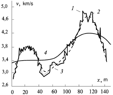
Let us consider the results of smoothing of stacking velocity along a profile.
At Fig. 8.1 the initial data and smoothing data at various values of the weighted
multipliers g
k
(the same for all points g
k
= DP ) are represented. From the analysis
of the curves it follows that at decreasing of the weighted multipliers from 1 to
0,0001 a transition from smoothing of high frequencies to low frequencies occurs.
Fig. 8.1 Smoothing of the effective velocity along profile by the cubic spline functions: 1 is initial
data, 2 — DP = 10
−1
, 3 — DP = 10
−2
, 4 — DP = 10
−5
.