Tennick A. Practical PowerPivot & DAX Formulas for Excel 2010
Подождите немного. Документ загружается.

14 Practical PowerPivot & DAX Formulas for Excel 2010
If you expand the Orders and the Order Details tables in the PowerPivot Field
List, you can see the two new columns you added using DAX: Year and Sales
Amount. Under the Products table, you can also see your new Category column.
It looks no different from the original imported columns. You are ready to build
your first PowerPivot pivot table (hosted in Excel) by adding columns.
12. Right-click Category under the Products table (not CategoryName under
Categories) and choose Add to Column Labels. You can also drag and drop to the
Column Labels drop-zone. Do the same for ProductName. Under the Customers
table, right-click Country and choose Add to Row Labels (yes, columns can
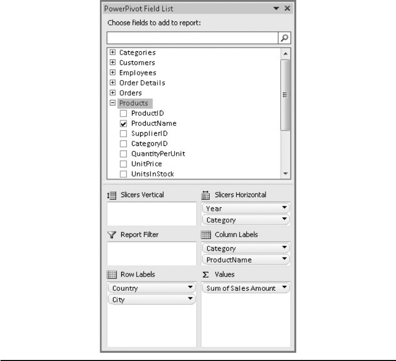
become rows!). Do the same for City. Under the Order Details table, right-click
Sales Amount and choose Add to Values. Next, under the Orders table, right-
click Year and choose Add to Slicers Horizontal. Repeat this for the Category
column in the Products table. There should be seven entries in the bottom half of
the PowerPivot Field List—by default, the lower section of the PowerPivot Field
List contains drop-zones for different areas of the pivot table. Category appears
twice, and Sales Amount (in the Values section) is named Sum of Sales Amount.
Your PowerPivot Field List should look something like Figure 1-15.
13. Now is probably a good point at which to save your work. You save from Excel as
you normally do, although you can also save from the PowerPivot window. Both
the Excel workbook and the PowerPivot model, including both metadata and
data, are saved as one single .xlsx file. You have just created a multidimensional
cube without having to know anything about star schemas or cubes or dimensions
or facts/measures or SSAS. If you copy the .xlsx file and rename with a zip
extension, you can unzip the file. It contains quite a lot! In the customData
subfolder of the xl folder, there’s a file called item1.data, which is fairly big. This
file is your PowerPivot data.
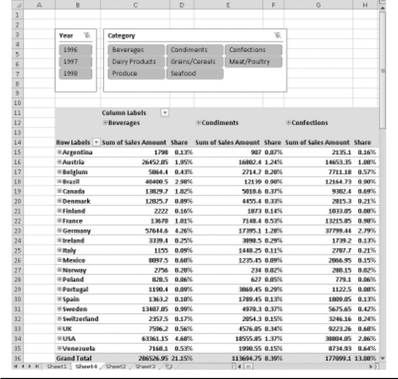
14. In the pivot table, right-click on Argentina under Row Labels and choose
Expand/Collapse, followed by Collapse Entire Field. Repeat this process for
Beverages under Column Labels. Your pivot table should resemble Figure 1-16.
That’s pretty good for a few minutes’ work, isn’t it? You might want to experiment
with expanding and collapsing the countries and the categories. Something you
may not have seen before are the two slicers at the top. Try clicking individual
years or product categories to implement filters and watch the data change (it’s
really fast). To select more than one filter in a particular slicer, click the first tile
and hold down the ctrl key as you click others—the data will not refresh until
you release the ctrl key. Or you can hold down the mouse button to select
contiguous slicer tiles. To show all of the data and clear any slicer filters, click the
small filter funnel (which has a red cross when a filter is in operation) at the top
right of a slicer.
Chapter 1: PowerPivot: Quick Start 15
This is a really cool pivot table. But we can make it even better. For example, there are
some blank cells, which you might wish to change to zeros—our Norwegian customers
are not keen on Grains/Cereals. Maybe the Sales Amount could be formatted a little
better. And it might be nice to show market shares by country/city and category/product,
as a percentage of the overall total sales (1354458.59 in the bottom-right corner). All of
this, and much more, can be accomplished with your mouse from the GUI— Chapter
5 goes into detail about pivot table possibilities. For example, you can exploit the power
of Excel’s conditional formatting capabilities. However, we are going to add some new
data to show percentage market share using DAX. When you work with cells in the
Figure 1-15 PowerPivot Field List with entries

16 Practical PowerPivot & DAX Formulas for Excel 2010
Values area, you are working with measures (sometimes referred to as facts). Measures are
usually numeric values that are used to show totals and subtotals—more on this later.
Earlier, you used DAX to add columns to tables—these are DAX calculated columns.
The second situation when we use DAX is to create measures. DAX formulas are either
calculated columns or measures. As you progress through the book, the difference
between calculated columns and measures should become clear. If you have star schema
experience, you can think of them as dimensions and facts. If you have cube experience,
you might know them as dimensions and measures. However, to use PowerPivot and
DAX, you don’t need any knowledge of either star schemas or cubes. The whole point
of PowerPivot for Excel is to shield you from such technicalities.
To create your first DAX measure:
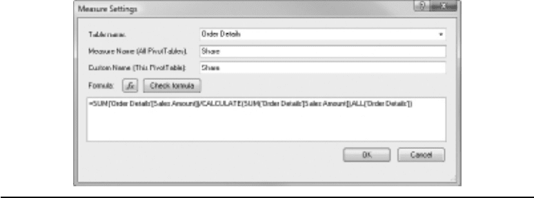
1. Click New Measure in the Measures group of the PowerPivot ribbon in the Excel
workbook. This opens the Measure Settings dialog box (Figure 1-17). If New
Measure is disabled, click inside the pivot table. An alternative is to right-click on
the table in the Field List and choose Add New Measure.
Figure 1-16 PowerPivot pivot table in Excel
Chapter 1: PowerPivot: Quick Start 17
2. Enter Share as the name for the new measure for Measure Name (All Pivot
Tables) and make sure that Order Details is selected in the Table name drop-
down. Then, enter the following DAX in the Formula box (if you need a bit more
room to type, expand the size of the dialog box and the Formula box will enlarge).
When you finish the entry, click Check Formula to verify your syntax.
=SUM('Order Details'[Sales Amount])/
CALCULATE(SUM('Order Details'[Sales Amount]),
ALL('Order Details'))
ere’s quite a bit going on here. Click OK to accept the DAX formula and it
should be added to the Values section. e new calculated measure, Share, also
appears under Order Details and has a calculator icon next to it. If it’s not in the
Values section, right-click the measure and choose Add to Values.
3. As a final, cosmetic step, let’s align our new Share measure and show it as a
percentage. Click on one of the values for Share in the main body of the pivot
table. Click PivotTable Tools, then click the Options tab to open its ribbon.
4. Check that the Active Field in the Active Field group is Share and click Field
Settings. This opens the Value Field Settings dialog. In this dialog, click the
Number Format button to open the Format Cells dialog. Select Percentage and
click OK twice. A quicker alternative is to right-click on one of the values in the
pivot table and choose Number Format. Well done, you have a really nice BI pivot
table—hopefully, it looks similar to Figure 1-18.
This was a short, quick chapter—but it covered a lot of ground. Despite the chapter’s
brevity, you’ve seen many of the important features and the versatility of PowerPivot for
Excel. If you tried the example, you have imported data into PowerPivot and created
some DAX calculated columns (and a DAX measure) to extend the data. In addition,
Figure 1-17 Measure Settings dialog
18 Practical PowerPivot & DAX Formulas for Excel 2010
you placed much of the data into a PowerPivot pivot table in Excel and saw just how
easy it is to build business intelligence. Please don’t be fooled by the small tables in
these examples—PowerPivot can handle millions of records in tables. This business
intelligence may be self-service and takes only a few minutes, but it’s truly industrial
strength. The next chapter consolidates what you’ve learned—it has more detailed
instructions. It also extends this chapter and shows how to import data from Access
and Excel and data feeds, as well as SQL Server again. The next chapter also shows
how to create relationships between PowerPivot tables, if they are not inherited from
your source data, which is always the case with Excel and data feed imports.
Figure 1-18 A completed business intelligence PowerPivot pivot table

PowerPivot: Overview
Chapter 2

20 Practical PowerPivot & DAX Formulas for Excel 2010
C
hapter 1 was a very quick introduction to PowerPivot for Excel. It concentrated
on importing data from SQL Server. This chapter takes a more detailed look
at importing data from SQL Server. It also shows how to import data from
Access, Excel, and data feeds. You are shown relationships between PowerPivot tables
and how to set them up, if they are missing. Data Analysis eXpressions (DAX) is used
to create both calculated columns in PowerPivot tables and measures in PowerPivot
pivot tables in Excel. In addition, a measure is added through the GUI, without the need
for DAX. You get to construct a sophisticated pivot table and a pivot chart linked to the
pivot table. Various ways of filtering data in a pivot report (pivot table or pivot chart)
are introduced.
This chapter consolidates and extends the example in the previous chapter. It should
give you a good overview of some of the main features and capabilities of PowerPivot.
Subsequent chapters build upon this chapter—in particular, the next chapter is a full
in-depth look at PowerPivot.
C
Key concepts Starting PowerPivot; importing data into PowerPivot from SQL
Server, Access, Excel, and data feeds; setting up relationships; DAX calculated
columns; DAX measures; pivot tables; pivot charts; filters; slicers
Starting PowerPivot
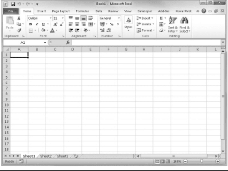
When you start Excel 2010, you are probably looking at the Excel Home ribbon as
shown in Figure 2-1.
If the Home ribbon is hidden, as in Figure 2-2, double-click the Excel Home
(or any) tab to re-enable ribbon display. If you single-click rather than double-click,
the ribbons are going to obscure the top part of your worksheet. If that happens,
try a double-click.
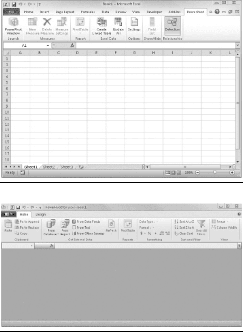
To display the PowerPivot ribbon, click the PowerPivot tab. The result is shown
in Figure 2-3. Maybe we should call this the Excel PowerPivot ribbon, as you’re still
in an Excel workbook. PowerPivot itself has its own separate window and ribbons, as
you’ll see in a minute. The PowerPivot ribbon has a number of groups. Presently, the
Measures, Report, and Show/Hide groups are disabled—these will become enabled
once you have added your first pivot table or created your first PowerPivot table.
When you create a pivot table from PowerPivot data, the pivot table is hosted within
an Excel worksheet. It is slightly different from a normal Excel pivot table, so it really
can be called a PowerPivot pivot table, although both can be seen in an Excel worksheet.
A PowerPivot pivot table (and/or a pivot chart) is where you visualize your Business
Intelligence (BI)—it’s your interface to your data. Perhaps I shouldn’t call it data any
more. Rather, it’s going to be information (meaningful data), or better still, intelligence.
Chapter 2: PowerPivot: Overview 21
Intelligence or business intelligence has many definitions. It’s information that is easily
found, easily visualized, and easily actionable. That means it’s going to form the basis for
sound and timely decision making. It gives you that competitive edge, and PowerPivot
makes it so easy!
If you don’t see a PowerPivot tab, and therefore you don’t have the PowerPivot ribbon, it
means you haven’t got PowerPivot! PowerPivot is not included with a default installation
of Excel 2010. Don’t worry; you can easily download PowerPivot for Excel for free. You
can find the download on the main PowerPivot Web site at www.PowerPivot.com, and it’s
also available from www.microsoft.com. Once you download and install, you should be
back with us with your PowerPivot ribbon open, as shown in Figure 2-3.
On the PowerPivot ribbon, in Excel, click the PowerPivot Window button—the
only one in the Launch group. This opens PowerPivot; see Figure 2-4. Veteran Excel
users may find this a little unusual. You now have two windows—the original Excel
workbook and the new PowerPivot window. Although they appear in two separate
Figure 2-1 Excel with ribbons

22 Practical PowerPivot & DAX Formulas for Excel 2010
windows, they are intimately related. When you save your Excel workbook in the
normal way, the PowerPivot window and its contents are saved as part of the Excel
workbook. Any data and settings inside the PowerPivot window are saved with
the Excel workbook. If you use the Save button in the Quick Access toolbar in the
PowerPivot window, it saves the outer Excel workbook and the PowerPivot window
within it. The PowerPivot window is not a separate workbook file that you can open
separately. If you have closed both windows, and you want to return to your PowerPivot
window, you open the Excel workbook first and click the PowerPivot Window button
on the Excel PowerPivot ribbon.
It’s easy to switch between the two windows. From the PowerPivot window, you
click the Switch to Workbook button in the Quick Access toolbar at the top. From
Excel, click the PowerPivot Window button in the Launch group of the PowerPivot
ribbon—this puts you back in the PowerPivot window. If this is the first time you’ve
clicked, it opens an empty PowerPivot window. If you had closed the PowerPivot
Figure 2-2 Excel without ribbons
Chapter 2: PowerPivot: Overview 23
Figure 2-3 PowerPivot ribbon in Excel
Figure 2-4 PowerPivot window
