Szilas A.P. Production and transport of oil and gas, Gathering and Transportation
Подождите немного. Документ загружается.

3
30
X
PlPt
1
INr
TRAN\PORTAl
ION
01
hATIIR4L
(>A\
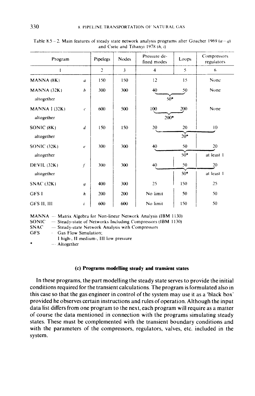
Table
8.5
-
2.
Main features
of
steady
state network analysis program.; after Coacher
1969
((I
~
y)
and
Csete
and Tihanyi
1978
(h,
i)
Program
I
MANNA
(8K)
MANNA
(32K)
Altogether
MANNA
I
(32K)
altogether
SONIC
(XK)
altogether
SONIC
I
32K)
Altogether
DtVIL
;32K)
altogether
SNAC
(32K)
GFS
I
GFS
11,
111
(I
h
I'
d
Y
1
4
h
1
Pipelegs
150
300
600
150
100
3ou
400
200
600
Nodes
3
I50
300
.-
500
150
300
300
300
200
600
No limit
50
50
No limit
I
150
I
50
MANNA
~
Matrix Algebra
for
Non-linear Network Analysis (IBM
1130)
SONIC
-
Steady-state
of
Networks Including Compressors (IBM
1130)
SNAC
~
Steady-state Network Analysis with Compressors
GFS
-
Gas
Flow
Simulation;
I
high-.
11
medium-.
111
low pressure
*
~~
Allogether
(c)
Programs modelling steady and transient states
In these programs, the part modelling the steady state serves to provide the initial
conditions required for the transient calculations. The program is formulated also
in
this case
so
that the gas engineer
in
control
of
the system may use
it
as
a 'black box'
provided he observes certain instructions and rules of operation. Although the input
data list differs from one program to the next, each program will require as a matter
of course the data mentioned in connection with the programs simulating steady
states. These must be complemented with the transient boundary conditions and
with the parameters of the compressors, regulators, valves, etc. included in the
system.

X
5
NUMtRlCAL
SIMLiLATION
OF
THI
FLOW
33
1
The main characteristics of some up-to date and
in
practice widely uscd programs
are listed
in
Table
8.5
-3
after Coacher
(1
969),
Goldwate:
c'r
ul.
(1
976)
and Tihanyi
(1980).
No mention is made in the Table of the General Electric's (USA) fairly
successful
GE Simulator program, since its characteristic data are not available.
This latter, similarly to CAP and ENSMP solves the differential equations
by
the
implicit method, whereas PIPETRAN and SATAN use the explicit method. As
a
matter of fact SATAN is the combinaiion
of
CAP and PIPETRAN. The three-
stage operation provides the program with high flexibility (see later).
For solving the basic equations the PAN algorithm uses the Crank-Nicholson
method. The program was tested partly by results obtained by the CAP method,
and partly by data telemechanically measured
in
a gas transmission network. The
correspondence was sufficiently good
in
both
of
the cases.
For solving the
differential equations the TGFS program uses a hybrid method that combines the
speed of the explicit and the stability of the implicit methods. Its principle is that at
each
At
time-step for the determination of the change in pressure at the nodes
it
calculates explicit and implicit steps respectively according to a previously defined
order. For an example as to the structure of a program simulating a complex gas
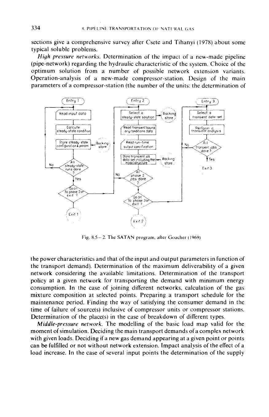
transmission system, let
us
consider that of SATAN.
The program consists of three main units, which may be run separately
if
so
desired.
-
Phase
1.
Calculation of the steady state. Quite often,
it
is necessary to
compare only the steady-state operation of various system configurations,
or
to
furnish initial conditions for the transient calculation.
In
that case, running this
program separately, one may examine up
to
I0
variants
in
succession.
At
the end of
each run, in addition to the printout of the desired results, all data required for the
transient calculation except the boundary conditions are stored
in
the background
memory from where
it
may be called in as and when required.
-
Phase
2.
This is the
connecting phase in which the transient model is built up step by step out
of
the
results of one
or
more variants of the previous phase, judged to be the most
interesting, and out of the boundary conditions fed into the machine. The results are
once more relegated to the background memory. Up to ten dynamic-model variants
may be stored also in this case.
-
Phase
3.
Transient analysis. The computer calls
in
the intermediate results, calculated in the foregoing phases, of one
or
several
preferred variants, and calculates the transient flow rates and pressures.
The block diagram of the program is given after Coacher in
Fig.
8.5-2. The
program structure is such that routines providing higher accuracy,
or
a faster
solution,
or
a more economical use of storage space can be introduced into the
program without changing its structure, merely by exchanging certain segments.
(d)
Programs solvable by simulation
In
the prefatory parts of the Sections
8.3
and
8.4
the application fields of the
steady state and transient flow simulation were discussed in general. The speediness
of the computerized design makes
it
possible that the programs, already known,
could be used for solving an ever increasing number of different problems. The next
w
w
N
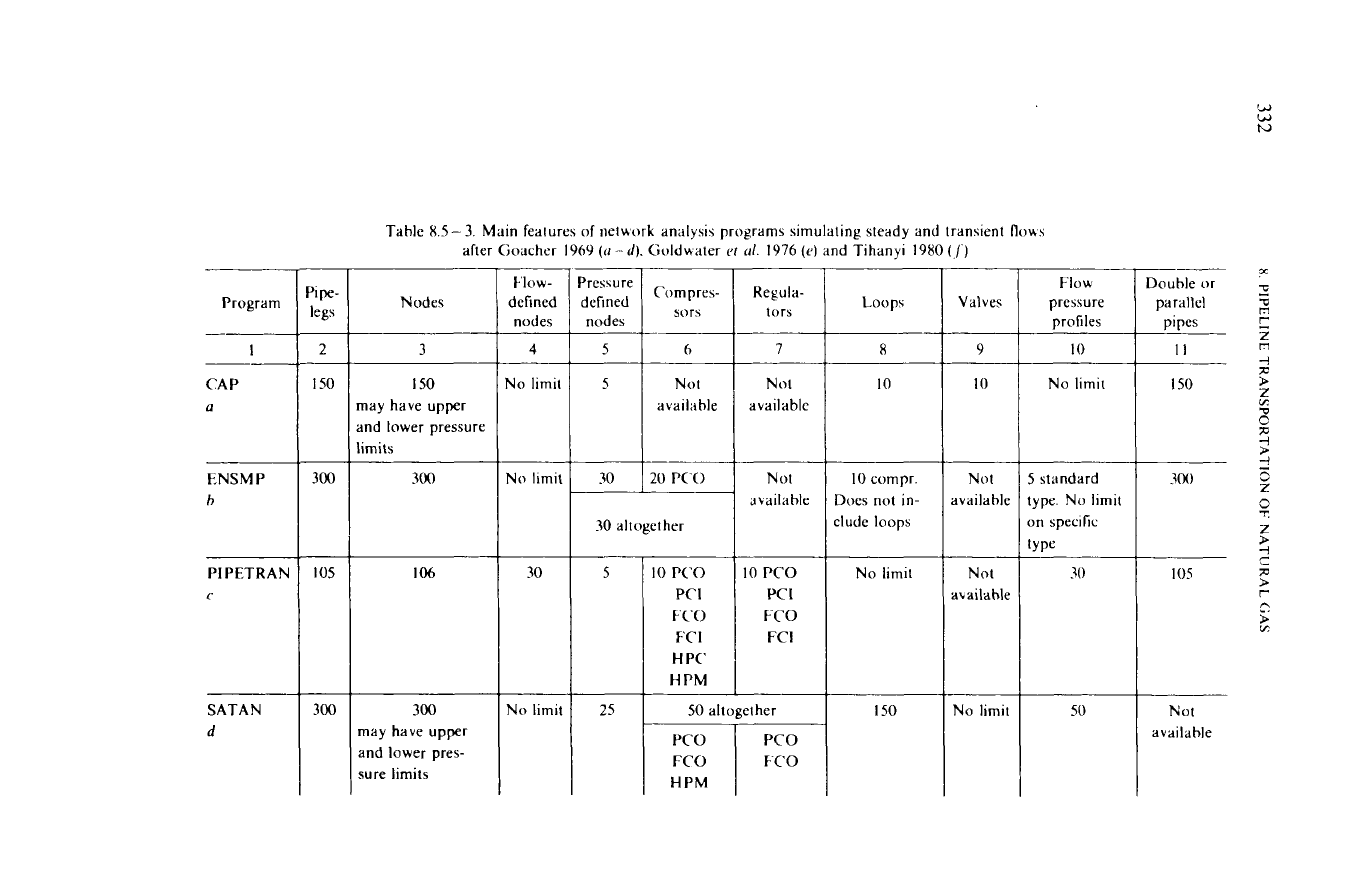
Table
8.5-
3.
Main features
of
network analysis programs simulating steady and transient
flows
after Goacher 1969
(ti
--
d).
Goldwater
('I
ti/.
1976
(el
and Tihanyi 1980
(/')
'ipe-
legs
Compres-
sors
Flow-
defined
nodes
4
Pressure
defined
nodes
5
Flow
pressure
profiles
10
Double
or
parallel
pipes
11
Regula-
tors
Program
I
____
Nodes
Valves
Loops
2
3
h
7
n
9
CAP
a
1
50
I50
nay have upper
md
lower pressure
imits
No
limit
5
Not
avaihhle
Not
available
10
10
No limit
1
50
ENSMP
h
300
-
I05
-
300
300
30
20
PC'O
10
compr.
Does not in-
:lude
loops
300
No limit
30
Not
available
10
PCO
PC
I
FCO
FCI
Not
availa
ble
Not
akailahle
5
standard
~ype. No limit
on specific
lYPe
30
30
altogether
PI PETRAN
c
106
No limit
5
10
PCO
PC
I
FCO
FC
I
H
PC'
H
PM
105
Not
available
SATAN
d
300
nay
have upper
dnd lower pres-
Pure limits
No
limit
25
I50
No limit
50
50
altogether
H
PM

PAN
e
TG
FS
I
215
200
400
200
No limit
No limit
-c_-
20
No limit
!5
PCO
PC
I
f
"0
H
PM
H
PC
No limil
PCO
PCI
FCO
H
PM
H
PC
No limit
~~
No limit
Not
ivailablc
~-
No limit
PCO
-
Pressure-controlled outlet
PCI
~
Pressure-controlled inlet
FCO
-
Flow-controlled
outlet
FCI
-
Flow-controlled inlet
H PC
~
Horsepower control
H PM
-
Horsepower maximum
ENSM
P
CAP
PIPECTRAN
-
Pipeline Transients, Electronic Associaieb Inc. (USA)
SATAN
PAN
-
Program
to
Analyse Networks, British Gas (Greal Britain)
TG
FS
-
Extended Network Systems Modelling Program; Engineering Research Station
of
Gas
Council (Fngland)
~
Control Advisory Program; Fnglneering Research Station
of
Gas
Council (England)
-
Steady and Transient Analysis
of
Networks; Gas Council, London Research Station
-
Transient
Gas
Flow
Simulation, Petroleum Engineering Ikpartment, TlIH
I
(Hungary)
99
w
w
w
sections give a comprehensive survey after Csete and Tihanyi
(1978)
about some
typical soluble problems.
High
pressure netnwks.
Determination of thc impact of a new-made pipeline
(pipe-network) regarding the hydraulic characteristic of the system. Choice of the
optimum solution from a number of possible network extension variants.
Operation-analysis
of
a
new-made compressor-station. Lksign of the main
parameters of a compressor-station (the number of the units: the determination of
T==+
Reud
input data
1
49
runs
done
I
Yes
t
Yes
EXIt
3
Fig.
8.5
-
2.
The
SATAN
program. afler Goacher
(
1969)
the power characteristics and that of the input and output parameters in function
of
the transport demand). Determination
of
the maximum deliverability of a given
network considering the available limitations. Determination of the transport
policy
at
a given network for transporting the demand
with
minimum energy
consumption.
In
the case of joining different networks, calculation of the gas
mixture composition at selected points. Preparing a transport schedule for the
maintenance period. Finding the way
of
satisfying the consumer demand
in
the
time of failure
of
source(s) inclusive of compressor units
or
compressor stations.
Determination
of the place(s) in the case of breakdown of different types.
Middle-pressure network.
The modelling
of
the basic load map valid
for
the
moment ofsimulation. Deciding the main transport demands of a complex network
with given loads. Deciding
if
a new gas demand appearing at a given point or points
can
be
fulfilled or
not
without network extension. Impact analysis of the effect
of
a
load increase.
In
the case of several input points the determination
of
the supply
X
6
PIPLLINE TRANSPORTATION
Or
NATbRAL
<,A\
335
districts belonging to different sources at nearly horizontal terrain and
if
the
network
is
created on a
hilly
surface with high level differences respectively.
Determination
of
the transport capacity increase due to the increased input
pressure. With several input points given the determination
of
the effect of the input
pressures’ change on the supply districts. Design
of
a network reconstruction.
Determination of the network extension’s impact on the hydraulic characteristics
of
the system. Impact analysis
of
the failure of a pipeleg.
In
the case
of
several sources
the analysis
of
the failure of a district pressure regulator
or
of some sources
respectively.
Low
pressure nerwork.
The analysis of network extending variants, the choice of
the optimum solution. The examination
of
the effect of a new district pressure
regulator. Determination of the heat transport capacity
of
a network when
changing from town gas to natural gas. Design of network reconstruction.
8.6.
Pipeline transportation
of
natural gas;
economy
In the previous Section, in connection
with
the flow simulation
in
gas
transmission network, the optimum variant was mentioned several times. Here
it
was tacitly assumed that we intended to choose the network and mode ofoperation.
that on one hand,
is
technically suitable to satisfy the consumer demands. and, on
the other hand
it
requires the minimum possible transportation costs.
It
has been
tacitly assumed too, that the gas volume demanded
by
the consumer
is
available at
the required rate and fixed price. Such assumption is imaginable for imported gas,
but not to such a degree
if
the source is a home gas field. The gas field and the gas
processing plant are also parts of the gas supply system in this case. Rentability can
also
be
influenced by the gas reserves of the fields. by the length of exploitation and
by the production rate. The orders, and complementary technical methods, by
which the daily
or
monthly rate of the production and transport can be stabilized all
year round can also have a great economic significance. This will be discussed
further on.
The duration of developing a gas field (drilling the gas wells, choosing the number
of producing wells, the preparation and transmission equipment to be matched to
them, the capacities and the construction and installation periods of these sets of
equipment) may vary rather widely. Mayer-Gurr illustrates the economic
importance of these factors on a simple example (Mayer-Gurr
1971).
Figure
8.6
-
1
(a)
shows the first two sections
of
the typical production curve of a gas field,
in
three variants. The exploitable gas reserve of the field was assumed to equal
55
km3.
Three rhythms of exploitation have been invisaged. The first production period
takes five years in
all
three.
It
is
during this period that production is run up to full
rated capacity. This latter is
4.5
km3 in the first case,
3-0
in the second, and
2.25
in the
third. This is the output that is desired to maintain over about
60
percent of the
field’s life. The period
of
level production is
10
years in the first case,
15
in
the second
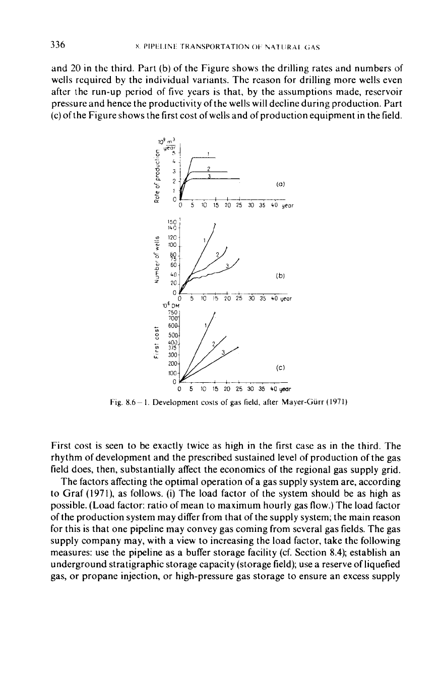
336
\I
I’Il’L1
11\11
rKAN\PORTATION
Ot
b471
RAI
(r45
and
20
in
the third. Part (b)
of
the Figure shows the drilling rates and numbers
of
wells required by the individual variants. The reason for drilling more wells even
after the run-up period
of
five years is that, by the assumptions made, reservoir
pressure and hence the productivity ofthe wells
will
decline during production. Part
(c)
of the Figure shows the first cost of wells and
of
production equipment in the field.
i
o__
0
5
10
15
20
25
30
35
30
35
40
year
Fig.
8.6-
1.
Development
cosis
of
gas
field.
after Mayer-Gurr
(1971)
First cost is seen to be exactly twice as high in the first case as
in
the third. The
rhythm
of
development and the prescribed sustained level
of
production of the gas
field does, then, substantially affect the economics
of
the regional gas supply grid.
The factors affecting the optimal operation
of
a gas supply system are, according
to Graf
(1971),
as follows.
(i)
The load factor of the system should be as high as
possible. (Load factor: ratio of mean to maximum hourly gas flow.) The load factor
of the production system may differ from that
of
the supply system; the main reason
for
this is that one pipeline may convey gas coming from several gas fields. The gas
supply company may, with a view to increasing the load factor, take the following
measures: use the pipeline as a buffer storage facility (cf. Section
8.4);
establish an
underground stratigraphic storage capacity (storage field); use a reserve
of
liquefied
gas, or propane injection,
or
high-pressure gas storage to ensure an excess supply
8.6.
PIPELINE TRANSPORTATION
OF
NATURAL GAS
337
capacity for periods of peak demand.
(ii)
Of
the above-enumerated measures, those
are taken that ensure the most economical solution in any given case.
(iii)
Gas fields
of various nature are
to
be
produced in the most economical combination, possibly
one after another.
(iv)
The system should ensure uninterrupted gas supply with a
high degree
of
safety. The safety of supply can be measured by two factors. One is
availability, which is the ratio of the aggregate length of uninterrupted supply
periods to total time. The other is the reserve factor. The higher the availability the
less reserve is needed in the form of parallel lines, underground storage capacity
or
standby peak-demand supply systems.
Underground storage in storage fields is a chapter of reservoir engineering. Here
we shall just touch upon the essentials and the nature of the procedure. Natural gas
may be stored in a gas reservoir, either exhausted
or
nearing exhaustion, in an
exhausted crude oil reservoir,
or
in an aquifer. Requirements facing a reservoir are
as follows.
(i)
It
should have a cap-rock impervious to gas,
(ii)
it
should have
sufficiently high porosity and permeability,
(iii)
the storage wells should not
establish communication between the formations traversed, that is, their casings
should
be
cemented in
so
as
to
provide faultless packoff (isolation);
(iv)
it
should
be
I
I
I
I
20
50
100
150
200
250
300
350
I
1
-
Fig.
8.6
-
2.
Natural gas supply (after Kridner
1965)
situated close to the area ofconsumption,
(v)
the reservoir rock should
be
chemically
inert vis-a-vis the gas to be stored.
-
The gas reservoir may
be
closed, with no inflow
of water from below
or
laterally. The storage space may in such cases
be
regarded in
a fair approximation as a closed tank whose volume equals the pore volume. In
open reservoirs, decrease of pressure entails the inflow of water from below
or
from
the periphery towards the centre of the reservoir. On the injection
of
gas into the
reservoir, the gas-water interface will sink. The gas-filled volume of this type
of
underground reservoir is, then, variable. In the USA, underground storage
reservoirs for the storage of natural gas have been in use since 191
5,
and G.
C.
Grow
(1965) predicted the volume
of
such reservoirs to attain
35
percent
of
country-wide
annual consumption by 1980.
22
338
X
PIPELINE TRANSPORTATION
OF
NATUKAL GAS
The main purpose of an underground storage reservoir is to mitigate the
economically harmful influence of seasonal fluctuations in demand. Such
fluctuations are significant especially where one of the foremost uses of gas is
in
heating. In order to exploit the capacities of the production and transmission
equipment more fully, a reserve is built up during the low-demand summer months
in underground reservoirs (storage fields) close to consumption centres. This is
where peak demand in the winter months is met from.
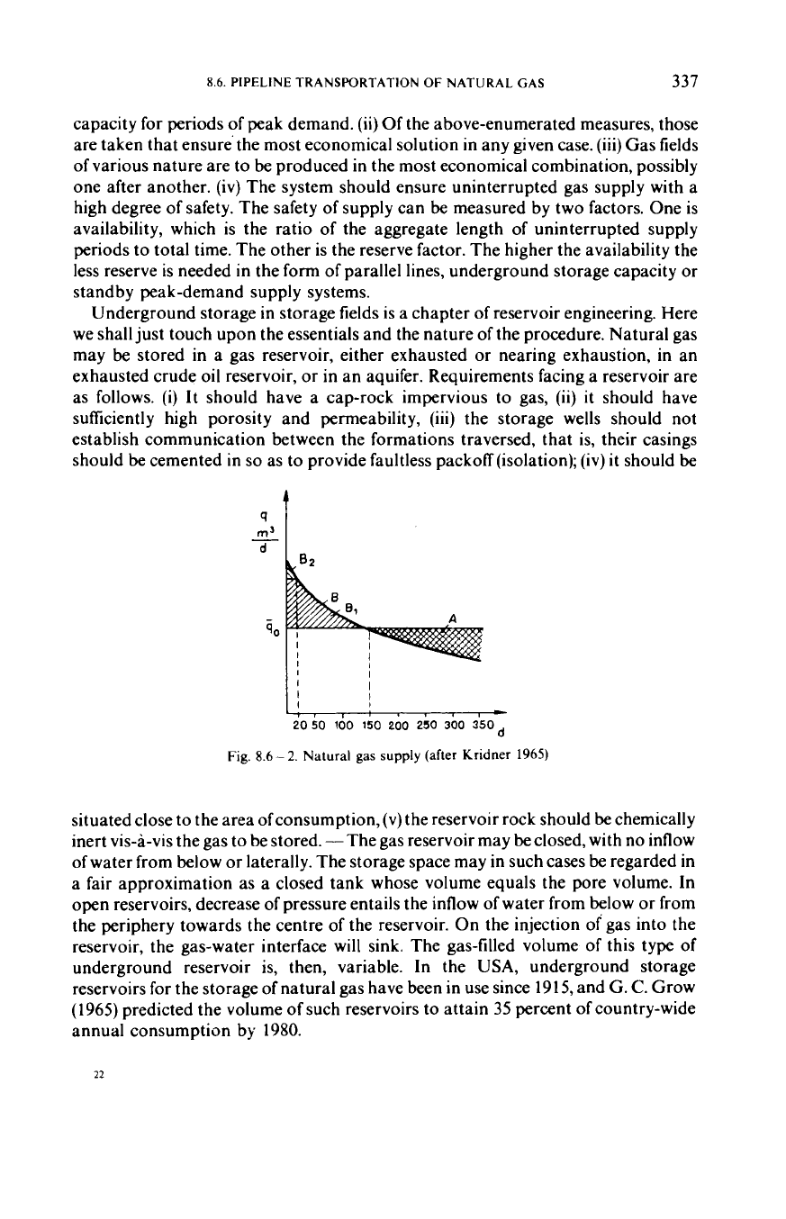
Figure
8.6
-2
is a typical diagram of natural-gas supply. The bold line shows the
number
of
days on which daily consumption exceeds some arbitrary daily
consumption
qi.
The area below the curve equals the annual gas consumption,
provided the axes are suitably calibrated. The average height of the area below the
curve equals the mean daily consumption,
Go.
Assuming that the production
equipment produces, and the transmission system conveys, a gas flow
qo
each day,
the area
A
indicates the volume
of
gas that can be stored up in the low-demand
period. Area
B,
equal to area
A,
is proportional to the volume of gas
to
be taken out
of
the reservoir on high-demand days. The diagram reveals that, in the case
2
0
Local protection
Tmlemmtering
Remote
control
-
Fig.
8.6
-
3.
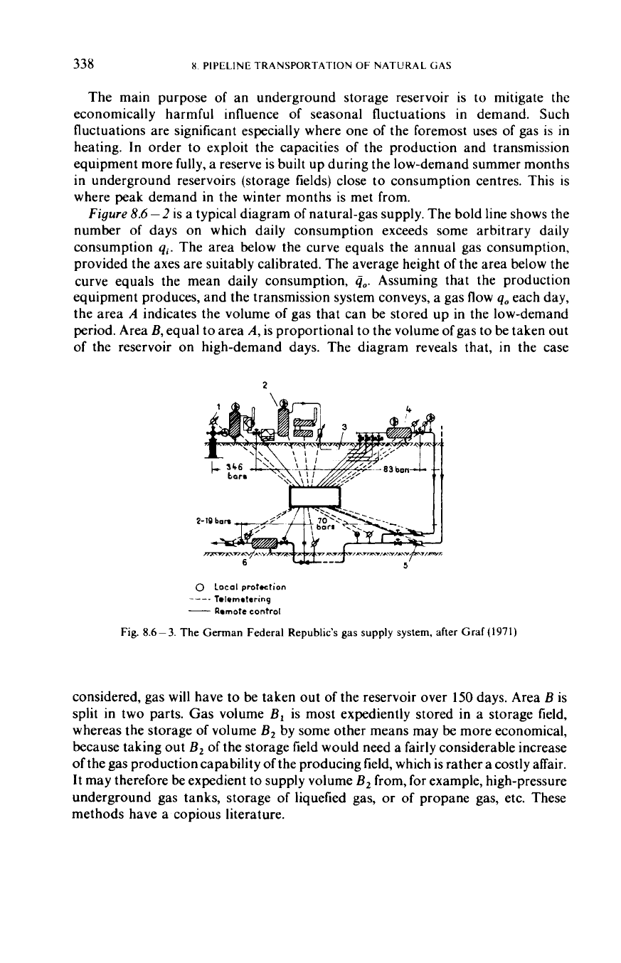
The
German
Federal
Republic’s
gas
supply system, after
Graf
(197
I)
considered, gas will have to be taken out of the reservoir over
150
days. Area
B
is
split in two parts. Gas volume
B,
is most expediently stored in a storage field,
whereas the storage of volume
B,
by some other means may be more economical,
because taking out
B,
of the storage field would need a fairly considerable increase
of
the gas production capability
of
the producing field, which is rather a costly affair.
It may therefore be expedient to supply volume
B,
from,
for
example, high-pressure
underground gas tanks, storage of liquefied gas,
or
of
propane gas, etc. These
methods have a copious literature.
8.6.
PIPELINE TRANSPORTATION
OF
NATURAL GAS
339
Regional gas supply grids are usually too complicated to be operated optimally
by unassisted men,
in
view
of
the continually changing demand and other
conditions facing the system. This is why the process control
of
such systems is
of
so
great an importance. Today’s consensus is that joint off-line control by man and
computer is to be preferred. One
of
the tasks
of
the computer is data acquisition and
the presentation in due time
of
adequate information. In possession
of
this
information, the dispatcher must be in a position to take optimal decisions and to
Production equipment Transmission equipment
Anaioqona
1
,,,/
frequency
multiplexing
-.-
Storage
Transmisslon
Reception
Cable
Reception
Tronsmis61on
Storage
.-
.-
Measurement Information Command
Fig.
8.6-4.
Information transfer, display and control (Mittendorf and Schlemm
1971)
Process
control
nth
16Kopemtiveme-
indruclicm
mory
rtomgc.15w
storoge
cycle
I
7
Interface
Electronic
Re
c e
I
ver
Remote- control
substation
Fig.
8.6
-
5.
Flow
of
information among telemetering, remote-control and program-control equipment
(Mittendorf and Schlemm
1971)
22.