Salcido A. (ed.) Cellular Automata - Simplicity Behind Complexity

Подождите немного. Документ загружается.

Equilibrium Properties of the Cellular Automata Models for Traffic Flow in a Single Lane

177

max max max

00 0

, ,

vv v

vvvv

vv v

nn vnq n

== =

∑∑ ∑

(2)

Here ε

stands for the kinetic energy of a particle with unit mass and speed v. It is easy to

show that flow q and kinetic energy ε of the system cannot exceed, respectively, the

maximum values q

max

(n) and ε

max

(n) given by

()

(1 )

max

⎧

⎪

⎨

−

⎪

⎩

0()

() 1

cmax

nnv

nv n

≤≤

≤

(3)

()

(1 )

max

⎧

⎪

⎨

−

⎪

⎩

0()

() 1

cmax

nnv

nv n

≤≤

≤

(4)

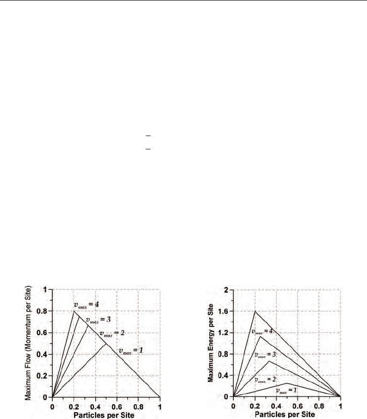
in the thermodynamic limit L→∞, where n

max

) is the critical density for v = v

max

. Diagrams

of q

max

(n) and

max

(n) are shown in Fig. 10. In the free-flow regime, n < n

max

), vehicles move

with speed v

max

, and the gap between vehicles is either v

max

or larger. In consequence, the

traffic flow in this regime is q

max

= nv

max

. If global density is larger than the critical density,

i.e. n > n

max

), only (L-N)/v

max

vehicles can move with maximum speed and, in the limit

L→∞, the maximum traffic flow is given q

max

= 1 – n. Similarly, it can be obtained the

maximum value ε

max

of kinetic energy for both n < n

max

) and n > n

max

). As a

consequence, the possible macroscopic states of the system are defined by those partial

densities n

which correspond to values of particle densities n and kinetic energies ε, ranging

in the intervals 0 ≤ n ≤ 1 and 0 ≤ ε ≤ ε

max

(n), respectively.

Fig. 10. Maximum flow q

max

(left) and maximum energy ε

max

(right) as functions of the

density of particles n, for models with v

max

= 1, 2, 3 and 4. For each n ∈ [0, 1], the possible

states of the system are those with energy ε ∈ [0, ε

max

(n)]. The transition points correspond to

the critical densities n

= 1/2, 1/3, 1/4 and 1/5.

Given initial and boundary conditions, the specific dynamical rules of the considered traffic

cellular automata will define the macroscopic state of the system at any time t.

Macroscopically, the state of the system will be characterized by the set of values of its

partial densities n

, or by the numbers N

= n

L, which is equivalent. Microscopically,

however, there are many different arrangements in the lattice of given numbers (N

, N

, ... ,

Cellular Automata - Simplicity Behind Complexity

178

vmax

) of particles moving there with speeds (0, 1, 2, ..., v

max

), respectively, including a

number Λ of sites which must remain empty. For models belonging to the GC-1DTCA, with

periodic boundary conditions, the number Ω(L, N

) of all these different microscopic

arrangements of moving particles is given by

()!

!!! !

max

NNNN

⎛⎞

Λ+

⎛⎞

⎜⎟

Ω=

⎜⎟

Λ+ Λ ⋅⋅⋅

⎝⎠

(5)

and the number of empty sites in the lattice (i.e., the lattice sites available for speeding up

the particles) can be expressed as

(1) 0

max

LvN

=− + ≥

∑

(6)

Negative values of Λ are forbidden because of the non-anticipation restriction that we

imposed to the models in the class we are considering.

We underline that Ω(L, N

) is the number of all the possible configurations in which we can

arrange N

bricks with 1-site length (representing the particles at rest), N

bricks with 2-sites

length (representing the particles moving with speed v = 1), N

bricks with 3-sites length

(representing the particles moving with speed v = 2), and so on, up to N

vmax

bricks with

max

+1)-sites length (particles with speed v

max

), by inserting them with no overlaps in a 1D

ring-shaped lattice with L sites in total, but allowing that a number Λ of sites remain empty.

We underline also that this result is valid for any cellular automata traffic model with all the

common features we have specified above (Section 2.2.1). However, since particular

dynamical rules of a model could prevent the system of reaching some microscopic states

with particular configurations of particles, Eqn. (5) will provide, at least, for such cases, an

upper bound to the number of them for that model.

Starting from Ω(L, N

), the entropy function is defined by S = ln(Ω). Then, with the help of

Stirling’s approximation, the entropy per site, s = S/L, in the thermodynamic limit (L→∞),

can be expressed as

( )ln( ) ln ln

max

sn n nn

λλλλ

=+ +− −

∑

(7)

where

1(1)

max

==− +

∑

(8)

As a pretty nice consequence of existence of entropy for the cellular automata traffic models

we are considering here, we can follow microcanonical equilibrium statistical mechanics to

find the equilibrium states of these models as the states that maximize the entropy for given

density and energy. These constraints seem suitable because cellular automata traffic

models involve rules with parameters (such as randomization p in the NS-model) that

control the kinetic energy of the particles, and drive the system towards macroscopic steady-

states with velocity distribution densities (and kinetic energies) well defined.

Equilibrium Properties of the Cellular Automata Models for Traffic Flow in a Single Lane

179

By employing the method of undetermined Lagrange multipliers, the velocity distribution

functions (or partial densities) n

which define the equilibrium states were obtained

βε

−−

⎛⎞

⎜⎟

⎝⎠

(9)

where  and β are Lagrange multipliers whose physical meaning is discussed in Section 5.

For v

max

= 1, Eqn. (9) leads to the following expressions for the partial densities n

and n

functions of n and a energy related parameter γ,

nnn

− (10)

114(1)

nnn

⎡

⎤

⎛⎞

⎢

⎥

=−− −

⎜⎟

⎢

⎥

⎝⎠

⎣

⎦

(11)

Parameter γ was defined in terms of the Lagrange multiplier β which, as we will see later, is

the conjugated variable of the global energy density (kinetic energy per site) of the system:

≡

(12)

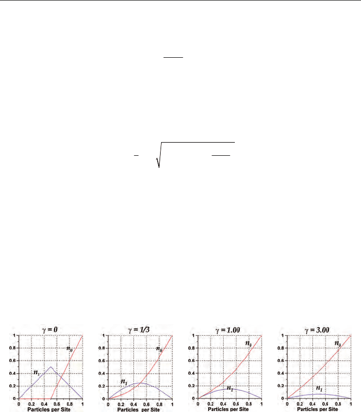
Traffic flow, in this case, is given by

q = n

. Diagrams of equilibrium partial densities n

and

are shown in Fig. 11 as functions of n for those models in GC-1DTCA with v

max

= 1, and

values

= 0, 1/3, 1, and 3. As can be seen, the equilibrium states we have found for

= 0 are

equivalent to the steady states of the WR184 model (and also to the steady states of the NS-

model with randomization

p = 0, and of the FI-model with stochastic delay p = 0). In fact, as

we will see later, the equilibrium states given by the equations (10) and (11) are completely

equivalent to the steady states of the NS-model with

max

= 1.

Fig. 11. Equilibrium partial densities

and n

as functions of n for models with v

max

= 1.

Traffic flow

q is the same as n

. The effect of the parameter

is appreciated clearly. The

equilibrium states of the models in GC-1DTCA with

max

= 1 and

= 0 are equivalent to the

steady-states of models WR184, NS (with randomization

p = 0), and FI (with stochastic delay

p = 0).

For

max

= 2, Eqn. (9) lead to the following equations for the velocity distribution densities:

012

nnnn

−− (13)

Cellular Automata - Simplicity Behind Complexity

180

(

)

(

)

()

12 1 2

nn n nn n

−− −−−

−−

(14)

(

)

()

112

nnnn

−− −

−−

(15)

Here, given

n and γ, the solution of Eqns. (14) and (15) give n

and n

, and then Eqn. (13)

gives

. This system of non-linear and coupled equations can be solved with standard

numerical methods (See, for example, Press et al., 1992). Here,

γ is the same as in Eqn. (12),

but now traffic flow, in according to Eqn. (2), is given by

q = n

+ 2n

. Numerical solutions

for the equilibrium partial densities

, n

and n

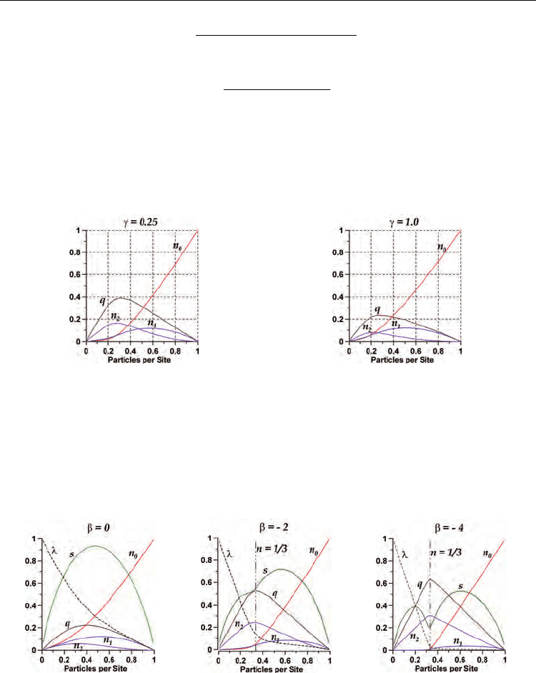
as functions of n are shown in Fig. 12.

Fig. 12. Equilibrium partial densities

, n

and n

as functions of n for models with v

max

= 2.

Traffic flow is

q = n

+ 2n

. The effect of the parameter

is appreciated clearly.

For

max

> 1, a singular behaviour of entropy at n = n

max

) (see Eqn. (1)) becomes evident in

the high-energy region (

β < 0). This is shown in Fig. 13 for v

max

= 2. For low energies (β > 0),

the state of the system corresponds to arrangements of particles with the three possible

speeds (

, n

> 0) for all densities 0 < n < 1. For high energies (β < 0), however, the

number of particles with speed

v = 1 behaves as a decreasing function of energy and dies

out in the high-energy limit (

β → - ∞). Just at this point, the entropy of the system comes out

(a) (b) (c)

Fig. 13. Equilibrium state entropy, flow and partial densities

, n

and n

as functions of n

for models with

max

= 2. The behaviour of entropy, as energy increases towards its

maximum

max

(1/3) = 2/3, shows a flow-regime transition at density n = n

max

) = 1/3, which

becomes sharper for higher energies.

Equilibrium Properties of the Cellular Automata Models for Traffic Flow in a Single Lane

181

clearly divided in two well differentiated parts: one for densities n < 1/3, and the other one

for densities

n > 1/3. The first part corresponds to free-flow states in the system, i.e., states

with all particles moving with the speed

max

= 2, and a number of empty sites λ > 0. The

second part corresponds to congested-flow states in which the system contains only

particles with speed

max

and particles at rest, and no empty sites (λ = 0). This behaviour of

entropy suggests a flow-regime transition in the system at density

n = n

max

) = 1/3, which

becomes sharper when energy increases towards the maximum energy (

max

(1/3) = 2/3).

4. Comparison with the steady states of the NS and FI traffic models

By comparing the simulation results shown in Figs. 4, 7 and 9, we can see that the NS and FI

traffic models with

max

= 1 are identical with each other, and to the WR184 model, in the

deterministic setting (i.e. when both the randomization in NS and the stochastic delay in FI

are set equal to zero). As it can be observed in the first diagram of Fig. 11, the same

behaviour is described by the equilibrium states for

= 0, case for which our equations (10)

and (11) are reduced to

nnn

−

114(1)nnn

⎡

⎤

=−− −

⎣

⎦

The NS and FI models, however, behave quite different each other when their respective

probability parameters, randomization and stochastic delay, are larger than zero. This is, of

course, what one can observe through the comparison of Fig. 7 against the diagrams shown

in Fig. 9 (first row). The equilibrium states in this case (

max

= 1, p ≥ 0), result expressed by

nnn

−

114(1)(1)nnnp

⎡

⎤

=−− −−

⎣

⎦

(16)

This result is the exact solution for the NS-model with

max

= 1 (Eqn. (5.11) in Schreckenberg

et al, 1995). It is obtained from Eqns. (10) and (11) once probability parameter

p is defined as

≡=

(17)

This is consistent, of course, with the meaning of the randomization probability

p in the NS

model because, as we will see later, the Lagrange multiplier

β is associated with the energy

of the system in such a way that β → - ∞ (β → +∞) corresponds to the high-energy (low-

energy) limit. In fact, we see that the high (β → - ∞) and low (β → +∞) energy limits

correspond to the randomization limits

p → 0 (no braking is allowed at all, and the particles

are driven to move with the possible highest speeds) and

p → 1 (each particle is obligated to

reduce its speed by one each timestep), respectively. In consequence, we are compelled to

conclude that the equilibrium states given by the equations (10) and (11) are completely

equivalent to the steady states of the NS-model with

max

= 1.

In Fig. 14, in terms of the partial densities

and the traffic flow q, it is shown a comparison

of the equilibrium states (solid lines) against computer simulations of the steady states of the

NS-model (dashed lines), considering

max

= 2 and randomizations p = 0.2 and 0.5. Here, for

each density

n we calculated the kinetic energy ε from the partial densities n

of the

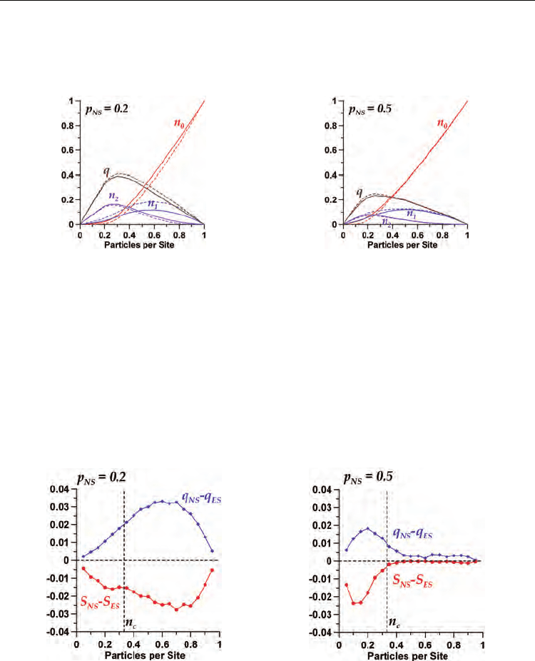
Cellular Automata - Simplicity Behind Complexity

182

simulated steady state. Then, for each couple (n, ε) we solved numerically the equations (14),

(15) and (16). As it can be seen, a reasonable qualitative and quantitative agreement between

the equilibrium states and the steady states of NS-model is found. However, growing

differences are observed as

p decreases below p = 0.5, particularly for densities n > 1/3.

Fig. 14. Comparison between the equilibrium theory results (solid lines) and computer

simulation results (dashed lines) carried out with the NS-model with

max

= 2, for

randomizations

p = 0.2 (left) and 0.5 (right). Although a reasonable agreement is found,

important differences are observed.

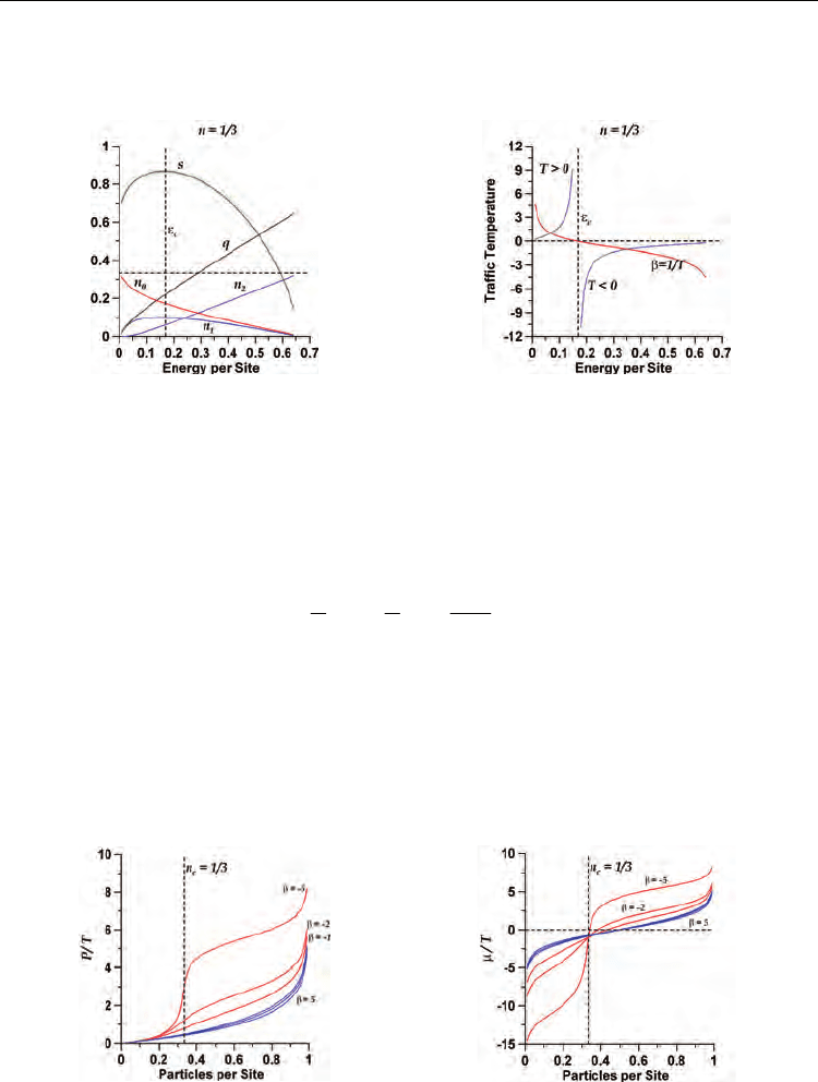
The observed differences are due to the rules implemented in the NS model for updating the

speeds of the particles, which give a non-equilibrium character to the NS-model. In Fig. 15

we have shown diagrams of the deviations of the values of flow

and entropy per site s

of the NS-model steady states with respect to the corresponding values

and s

of the

equilibrium states, for

p = 0.2 and p = 0.5. In both cases, the NS steady-state flow deviations

are positive, i.e.,

is larger than q

for any density n. For the entropy per site, however,

also for any density, the values

we calculated with the partial densities of the steady

states are lesser than the values

we calculated from the equilibrium ones, i.e. the

Fig. 15. Deviations of the NS steady state values of traffic flow

q (top) and entropy per site s

(bottom) with respect the corresponding equilibrium theory values, for p = 0.2 (left) and 0.5

(right). In both cases, the NS steady-state flow is larger than that one of equilibrium. For the

entropy, however, for any density

n, the values calculated with the partial densities of the

steady states are smaller than those calculated with the equilibrium ones. This result (we

think) is just an expression of the non-equilibrium behaviour of the NS traffic model.

Equilibrium Properties of the Cellular Automata Models for Traffic Flow in a Single Lane

183

deviations s

- s

are negative. This result is exactly what we expected because of the non-

equilibrium behaviour of the NS cellular automata traffic model. On another hand, as we

see in these figures, for

p = 0.2, the absolute deviations |s

- s

| for density values n > n

(congested flow regime) are larger than for

n < n

(free-flow regime); while for p = 0.5, on the

contrary, the absolute deviations for

n < n

are larger than for n > n

. Furthermore, for p = 0.5

the system behaviour in the NS-model is very close to equilibrium when

n > n

. This is due,

of course, to the braking effect of the randomization parameter, which forces a better

spreading of the particles among their possible speed values.

5. Equilibrium thermodynamic properties of 1D traffic cellular automata

In order to get some insight about the physical meaning of the Lagrange multipliers α and β,

we note that, using Eqn. (9), the entropy can be written as

(ln) ln

αλβε

⎛⎞

=+ ++

⎜⎟

⎝⎠

(18)

Now, a formal comparison of this equation with the well-known Euler equation of

thermodynamics for a gas of particles,

TTT

−++

(19)

where

s is the entropy per unit volume, n is the density of the number of particles, T is the

temperature, µ is the chemical potential, ε is the internal energy per unit volume, and

P is

the pressure, suggests the following thermodynamics interpretation

⎛⎞

=− +

⎜⎟

⎝⎠

(20)

(21)

⎛⎞

⎜⎟

⎝⎠

(22)

Strictly speaking, Eqns. (20) and (21) just define the new parameters

T and µ in terms of the

Lagrange multipliers

and

, and equation (22) defines P. However, the use of these

properties, which we will call traffic temperature (

T), traffic chemical potential (µ), and

traffic pressure (

P), could open an innovative framework for the physical analysis and

interpretation of traffic flow phenomena.

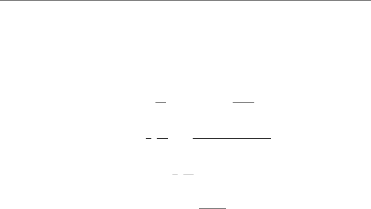
Traffic temperature (

T = 1/

) may assume positive and negative values, with a discontinuity

at the kinetic energy

where entropy reaches its maximum (Fig. 16), and splits the energy

spectrum in a low (

T > 0) and a high (T < 0) energy regions. This feature of temperature

(also inherited by the traffic pressure and chemical potential) is a typical consequence of the

upper bound imposed on the kinetic energy of the lattice gas particles (Salcido & Rechtman,

1991; Bagnoli & Rechtman, 2009), and it points out the existence of a population inversion of

the particles between the low and high kinetic energies. In fact, as it is suggested by Fig. 16,

Cellular Automata - Simplicity Behind Complexity

184

as n → n

max

) = 1/3, entropy is zero when all the particles are at rest (n

= n); reaches its

maximum value when the numbers of particles at rest and particles in motion are equal:

+ n

; and becomes null again when all particles are moving with speed v

max

= n).

Fig. 16. (Left): The entropy per site (

s), flow (q) and partial densities n

are shown as

functions of energy per site (

) for the critical density n = n

max

) = 1/3. Observe the typical

behaviour of entropy for systems with an upper bound in energy. (Right): Temperature,

defined as the slope of entropy as function of energy, has positive values for energies

and negative values for

, being

the energy at which entropy reaches its maximum.

It is interesting the behaviour of traffic pressure in the limits

n → 0, n → 1, and n → n

max

For the first two limits, respectively, the Eqn. (22) gives

≈

⎛⎞

≈

⎜⎟

−

⎝⎠

(23)

The result of the first limit (

n → 0) resembles the well-known equation of state of an ideal

gas. In the second one (

n → 1), depending on the s of temperature, P→±∞; this result

resembles the behaviour of pressure-density relation in a condensed phase. For high

energies

(

→ - ∞), the same as with entropy, traffic pressure and chemical potential have a

peculiar behaviour in the limit

n → n

max

). This is shown in Fig. 17 for speed limit v

max

= 2.

In both cases, this behaviour is a result of the singularity these properties have at

= 0. In

the high-energy limit, the density of empty sites dies out (

→ 0) when density n increases

Fig. 17. Properties

P/T and μ/T as functions of density n for several values of β. These plots

suggest a critical behaviour of traffic flow near

n = n

max

) = 1/3 in the limit of high energy

(β → -∞) of the system with

max

= 2.

Equilibrium Properties of the Cellular Automata Models for Traffic Flow in a Single Lane

185

towards n

max

), and so P/T and

/T diverge to infinity as ln(1/

). Because

remains null for

densities larger than

max

) (see Fig. 13c), P/T and

/T will remain undefined there.

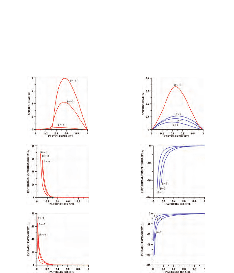
Other thermodynamic properties, such as the specific heat

, isothermal compressibility

and isobaric expansivity

, can be calculated easily from the velocity distribution densities.

The expressions we have obtained for these thermodynamic properties are shown in the

equations (24), (25) and (26). The behaviour of these properties is shown in Fig. 18.

max

222

()

ββε

⎛⎞

∂

≡− = −

⎜⎟

∂

⎝⎠

∑

(24)

(,)

(1)(1)

ee n

ββ

νβ

κβ

∂

⎛⎞

≡− =−

⎜⎟

∂

−

−−

⎝⎠

(25)

(,) (,)

PPP

αββ βκβ

νβ

⎛⎞

∂

≡− =

⎜⎟

∂

⎝⎠

(26)

with

νλ≡−=−

−

(27)

In this figure, we can observe the effect on the thermodynamic properties due to a sharp

transition between the free- and congested-flow regimes. In particular, it is observed that

compressibility and expansivity go to zero as n is increased towards 1/3. This means that for

n > 1/3, in the high-energy limit, no empty sites will be available in the lattice in order to set

in motion the particles at rest (i.e., the system of particles cannot be expanded), and any

particle will be found at rest or moving with the speed v

max

. This behaviour of particles in

the high-energy limit is observed also in the Fig. 13.

6. Conclusions and future work

The cellular automata traffic models of Nagel-Schreckenberg (NS) and Fukui-Ishibashi (FI)

include velocity updating-rules which define a dynamics that do not obey a detailed

balance. These rules continuously drive the system to states out of equilibrium. This is the

reason why these models and their variants cannot be studied within the framework of

equilibrium statistical mechanics. Nevertheless, as we have shown here, thermodynamic

entropy exists for the 1DTCA models with no velocity anticipation, which we have found

through an isomorphic system where a lattice gas particle which moves with speed v is

modelled as a brick, (v+1)-sites length, that is inserted in a 1D lattice with no overlapping.

This allowed us to study the equilibrium (or maximum entropy) states of these systems and

their thermodynamic properties. As it could be expected, the maximum entropy states do

not agree in general with the steady states of the NS model, particularly for high energies

(i.e. small values of the randomization parameter p); however, in the low energies domain

the equilibrium states resemble very strongly the steady states of the NS model, and the

fundamental diagrams are reproduced quit well. For v

max

= 2, the behaviour of entropy, as a

function of the density of particles, allowed a clear identification of different flow-regimes in

the 1DTCA models, displaying a sharp transition between the free- and congested-flow

regimes in the high-energy limit. The presence of this transition was observed also in other

Cellular Automata - Simplicity Behind Complexity

186

properties of the system, such as the specific heat, the isothermal compressibility, and the

isobaric expansivity, which were calculated using the velocity distribution densities of the

equilibrium states. Therefore, we presume that the knowledge of thermodynamic properties

within the context of modelling traffic flow by means of cellular automata is quite relevant

for improving and speeding up the computer simulation of traffic flow, but also may help

us to improve the physical understanding of traffic flow phenomena. So, we hope this work

may contribute in advancing some modest steps in the establishment of the traffic cellular

automata theory.

(a) (b)

(e) (f)

Fig. 18. Behaviour diagrams of the thermodynamic properties of the 1DTCA models with

max

= 2, for

< 0 (left column) and

> 0 (right column). First row: Specific heat C

. Second

row: Isothermal compressibility

. Third row: Isobaric expansivity

. All the properties

were plotted as functions of the density of particles n. For

< 0 these diagrams show the

occurrence a flow-regime transition at density n = n

max

) = 1/3.