Research on oil recovery mechanisms in heavy oil reservoirs

Подождите немного. Документ загружается.

268

269

Table 1. Comparisons of Calculated

p ’s at Various

Values of

r and

t for Closed Systems

r 5=

()

∞

()

pss

()

∞

()

pss

0.20 0.4241 0.427 0.4489 3.0 1.1665 1.167 1.2255

0.30 0.5024 0.507 0.5156 4.0 1.2750 1.281 1.3088

0.40 0.5645 0.579 0.5823 5.0 1.3625 1.378 1.3922

0.50 0.6167 0.648 0.6489 6.0 1.4362 1.469 1.4755

7.0 1.4997 1.556 1.5588

10.0 1.6509 1.808 1.8088

10=

()

∞

()

pss

15 1.8294 1.832 1.8973

20 1.9601 1.968 1.9983

30 2.1470 2.194 2.2003

40 2.2824 2.401 2.4024

50 2.3884 2.604 2.6044

Comparisons of

p ’s at

100=

Closed Outer Boundary (Katz et al., 1968)

()

∞

()

pss

100 2.7233 2.723 3.8760

250 3.1726 3.173 3.9060

500 3.5164 3.516 3.9560

1,000 3.8584 3.861 4.0560

2,500 4.3166 4.335 4.3561

5,000 4.6631 4.856 4.8561

10,000 5.0097 5.856 5.8562

25,000 5.4679 8.857 8.8569

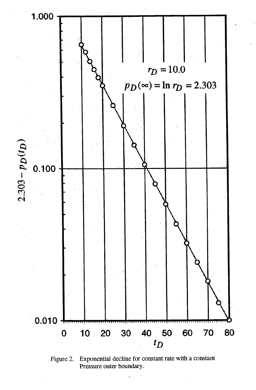
If we look at these results in detail, certain trends and comparisons become obvious. First,

the infinite system tables show the smallest pressure drops, but at early times the pressure behavior

for the finite systems closely follows that of the infinite system. The pseudo-steady state equations

predict the greatest pressure drops. But again, note that the later time behavior of all the real

systems closely follow the pseudo-steady state equations.

A most important conclusion can be reached by evaluating the tabulated data in detail. We

see that one or the other of these simpler equations will predict the values in the tables with an error

of only about 1% over the entire range of data. In brief, the tables for finite systems are not needed

at all! We can use the infinite system equations at early times and then switch to the pseudo-steady

state equation to calculate for later times.

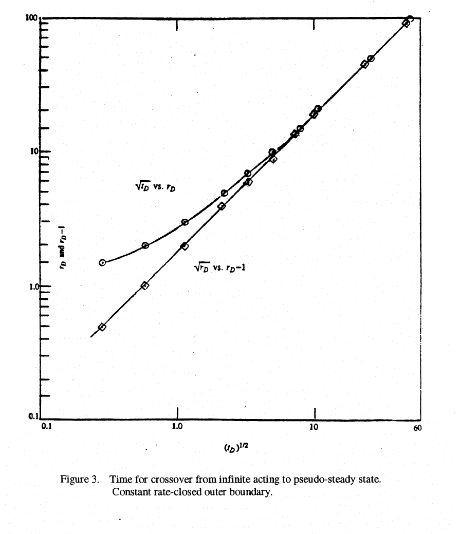
To carry the idea out in detail, I have performed these same calculations for a host of

’s

ranging from 1.5 to 100, and have evaluated the

t ’s at the crossover times. These results are

shown in Fig. 3 as circles. These data were straightened by graphing against

1−

r rather than

r .

270

The resulting data are shown as diamonds on Fig. 3. They clearly fall on a straight line,

whose slope is almost equal to 1.00. The equation is ,

945.1

)1(328.0 −=

rt (15)

In summary, to make calculations for a closed system at constant rate; at early times the

equations for an infinite system can be used, and at late times, Eq. 14 can be used. Equation 15

defines the time,

t , to switch from early to late time calculations.

Constant Pressure Inner Boundary

For the constant rate cases, Chatas looked at three outer boundaries: infinite, closed and

constant pressure. For the constant pressure case, in Table 2, he lists the infinite system, and in

Table 3 he lists closed outer boundaries. He did not look at the constant pressure case. It is not

too important to consider this case, so we’ll ignore it, and begin by looking at the infinite system in

Chatas’ Table 2, and also at Elig-Economides more recent work, (Appendix B) which is more

accurate.

Infinite Aquifer

Note the headings in Chatas’ Table 2 for the infinite aquifer. Dimensionless time is labeled,

t, while we commonly use

t now. The fluid influx term is labeled

()

tq . This is cumulative

influx, and the present nomenclature is

()

tQ . Dimensionless influx rate is not listed in this

table, but we will discuss this later, and its symbol is now

()

tq .

For the constant rate inner boundary, we noted that the very early time data closely followed

the

()

2/1

t equation. This is also true for the constant pressure case. It seemed likely that this idea

could be extended empirically by adding a term using

t to some other power. The following

equation was found to fit the tabulated data for

0.1001.0 ≤≤

t ,

()

90.02/1

510.0058.1

DDDD

tttQ += (16)

The fit is quite accurate over this range. The values at

01.0=

t and 0.05 show rather large errors

of up to 2.5 %, but these are usually not too important in practical use. Further, there is likely

some inherent error in Chatas' table for these low values of

t for they do not quite behave

logically. The rest of the data show errors of 1% or less.

At late time, it seemed likely that a semi-logarithmic approach would work,

()

tba

ln+= (17)

It does! However, we would like to extend this equation to a shorter time range. I added an

emperical constant to the

t on the left-hand side of Eq. 17, as follows,

()

ln4887.00407.0

4.1

−

(18)

This equation fit Ehlig-Economides' data from

0.10=

t to 000,100=

t , with a maximum error

of 0.40%; very good indeed.

Closed Outer Boundary

In thinking about a closed outer boundary, with a constant pressure inner boundary, we should

realize that, after a period of time, water influx will stop. This will occur when the entire

271

272

aquifer has been depleted to the inner boundary pressure. We can calculate the maximum

cumulative influx using simple material balance principles, as follows,

()

−

=∞

(19)

The long time results in Chatas’ Table 3 verify this equation.

The early time data in these tables also behave logically. We would expect that, at early

time, the effect of the outer boundary would not be felt. So the finite systems should act the same

way as an infinite system. They do! This is why Chatas started his listings in Table 3 after a period

of time.

Ehlig-Economides (1979), in her Ph.D. dissertation, looked at the flow behavior for a

constant inner boundary pressure. One important conclusion she reached was that all the finite

systems exhibit exponential decline once the outer boundary is felt. It is interesting that neither van

Everdingen and Hurst (1949) nor Chatas recognized this fact. I’ll show how this idea can be used to

tranform Chatas' results into simple equation forms.

For any finite system, after a time, the flow rate at the inner boundary is proportional to the

difference between the average pressure and the inner boundary pressure, as follows.

()

[]

()

tdQ

ptpC

≡

−

(20)

Also, we can define cumulative influx, using the material balance as follows,

()

[]

()

tppC

−

)( (21)

We can now combine Eqs. 20 and 21, rearrange and integrate, to get,













−

)(

tQC

(22)

Next we need to evaluate the constants,

C and

C in Eq. 22. At time, 0=t , 0)( =tQ ,

and from Eq. 20 and Eq. 21, we can define

C ,

)0()( Cqtq == (23)

When

∞=t , the log term in Eq. 22 must be infinite, so we can conclude,

)()( CQtQ =∞= (24)

As a result, Eq. 22 becomes,

()













−∞

∞∞

tQQ

)(

)0(

)(

(25)

Equation 25 is only valid from the time when exponential decline begins. However we can

extrapolate the equation back to

0=t , and it can be changed to the following dimensionless form,

which is not quite correct, but very nearly so.

273













−∞

−∞−∞

)()(

)0()(

)0(

)0()(

DDD

tQQ

(26)

It only remains to evaluate these terms from the data in Chatas’ tables.

The evaluation problem is more difficult than it first seems. It requires a number of

graphical procedures and calculations, plus some correlation work to correct for the slight errors

involved in getting from Eq. 25 to Eq. 26. The procedure I used was as follows. First I graphed

[]

)()(

DDD

tQQ −∞ from Chatas’ Table 3 against

t on semilog paper, as suggested by Eq. 26.

The straight line portions of these graphs were extrapolated to

t . These are the correct values

[]

)0()(

QQ −∞ for Eq. 26. After all of Chatas’ tables had been evaluated, an empirical

equation was derived to calculate

)0(

Q . It was a function of

rr / , as expected.

Finally, I evaluated the slopes of the semilog straight lines, and compared them to the slopes

one would calculate using pseudo-steady state for the terms in front of the logarithm in Eq. 26.

There was a slight error since the flow is not quite pseudo-steady state, which I correlated against

rr / .

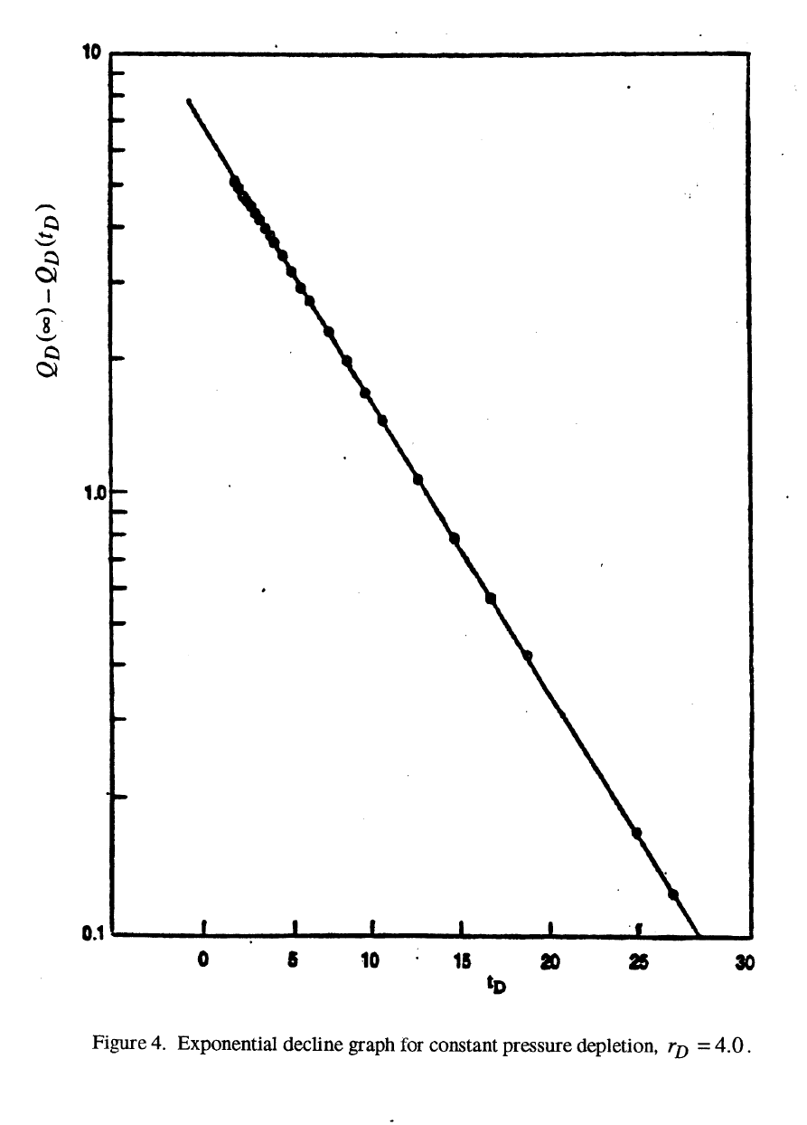
Since all this procedure may be a bit hard to follow, I’ll show a detailed set of example

calculations, for

0.4=

r , to show the procedure. For 0.4=

r , from Eq. 19, we can calculate

)(∞

Q , as follows.

500.72/]1)0.4[(2/]1)/[()(

=−=−=∞

weD

rrQ (27)

The data from Chatas’ Table 3 are graphed in Fig. 4. It is clear they fit a semilog straight

line. To evaluate the slope, I used values from his table at

0.2=

t and 0.26=

t .

00.2=

t , 442.2)( =

tQ ; 058.5)()( =−∞

tQQ

0.26=

t , 377.7)( =

tQ ; 123.0)()( =−∞

tQQ

The slope is,

4576.6

)123.0(ln)058.5(ln

00.20.26

)]0.26(ln[)]00.2([ln

−

∆−∆

∆

(28)

Using the slope from Eq. 28, and the value of

)00.2()(

QQ −∞ equal to 5.058, the value of

)0()(

QQ −∞ can be easily calculated,

)058.5(ln

4576.6

00.2

)]0()([ln +=−∞

8942.6)0()( =−∞

QQ (29)

Thus the value of

)0(

Q for this

r )0.4( =

r is,

6058.08942.6500.7)0( =−=

Q (30)

The values of

)0(

Q for all the radii were correlated into the following equation.

(0) = 0.013 + 0.1756 (r

−1)

1.111

(31)

Next I calculated the approximate value for

)0(

q assuming the pseudo-steady state

equation was valid. This equation (Brigham, 1998) is,

274

9787.0

1)0.4(

)4(ln)0.4(

)0(

=−

−

=−

−

(32)

Thus the approximate value for the slope is,

7474.6)9787.0(8942.6

)0(

)0()(

−∞

(33)

The actual slope is Eq. 28, while the approximate slope is Eq. 33. The error is thus,

Slope Error

045.1

4576.6

7474.6

(34)

The values of these errors were correlated into an equation for all radii, as follows,

Error =

1.070

−

057

−

0.297

(35)

In brief then, we now know we can calculate the early time constant pressure aquifer data

using Eq. 16 or Eq. 18, depending on the time range, and we can calculate the later time (depletion )

history using Eqs. 26, 33 and 35. It only remains to define the time to switch from infinite-acting to

finite-acting (depletion) behavior. Again this required correlating the data in Chatas’ Tables 2 and 3

as a function of

. The equation I came up with was,

21.2

)1(1600.0)( −=

DswitchD

(36)

Equation 36 is not very accurate. The reason, is that for all

’s, the infinite-acting data and the

finite-acting data were quite close to each other over a rather broad time range. Thus the precise

times could not be defined accurately. This, of course, is good news, for it means that all the

resulting calculations would be reasonably accurate.

To evaluate the accuracy of these equations at the times when we switch from infinite acting

to finite acting behavior, I have listed all the influx values from Chatas’ tables and from my equations

in Table 2. In this table, the first column shows all the

’s (

values) listed in Chatas’ Table

3. The second lists the switchover times calculated by Eq. 36; while the third column shows the

actual times used. These are near the calculated times, and also compatible with Chatas’ tables.

Table 2. Influxes From Chatas’ Tables 2 and 3

Compared to Approximate Equations

∞ Acting

Q Finite Acting

Calc.

switchD

t )(

Eq. 36

switchD

t )(

Used

Eqs. 16

and 18

Chatas’

Table 2

Eq. 26 Chatas’

Table 3

Max.

Diff.

(%)

1.5 0.035 0.050 0.2710 0.278 0.2753 0.276 2.58

2.0 0.160 0.15 0.5022 0.520 0.5064 0.507 3.54

2.5 0.392 0.40 0.8927 0.898 0.8940 0.897 0.59

3.0 0.740 0.70 1.255 1.251 1.257 1.256 0.46

3.5 1.212 1.00 1.568 1.569 1.574 1.571 0.56

4.0 1.814 2.00 2.448 2.447 2.443 2.442 0.24

4.5 2.55 2.50 2.836 * 2.836 2.835 0.04

5.0 3.43 3.50 3.554 * 3.552 2.542 0.34

6.0 5.61 6.0 5.150 5.153 5.144 5.148 0.17

7.0 8.39 9.0 6.859 6.869 6.853 6.861 0.23

8.0 11.80 12.0 8.446 8.457 8.436 8.431 0.31

9.0 15.85 15.0 9.970 9.949 9.932 9.945 0.38

10.0 20.6 20.0 12.36 12.32 12.29 12.30 0.57

275

276

The fourth and fifth columns compare the

Q ’s for the infinite acting system. The fourth

column is from my Eq. 16 for

’s up to 7.0, and from Eq. 18 for the three larger

’s; while the

fifth column lists the results from Chatas’ Table 2 for these same times.

The sixth and seventh columns show the same kind of information for the finite systems.

The sixth column shows the predicted values of

Q from Eq. 26, while the seventh column shows

values listed in Chatas’ Table 3. It is important that, at any

, all four values of

Q are very

close to each other. To compare them in detail, I’ve listed the maximum differences in the

listings in the eighth column. Note that the first two show differences of 2.58 and 3.54%, while all

the others are less than 1% in maximum difference. This is a remarkably accurate result!

The final evaluation is to compare the calculated exponential decline slopes (using all the

material discussed here) with the slopes found from Chatas’ Table 3. The equation

for the decline using my method is as follows,

Calculated Slope

)()0(

)0()(

Errorq

−∞

(37)

The decline rates calculated for these systems are quite accurate. The maximum error is 0.71%.

Linear Geometry

The behavior of a linear aquifer is far simpler than a radial aquifer. The mathematics of the

problem were first published by Miller in 1962, but shortly after that a quite elegant piece of work by

Nabor and Barham (1964) presented the entire linear aquifer equations and curves in a three-page

paper. The remarkable result of Nabor and Barham’s work was to show that all six possible

boundary conditions (Interior Boundary, constant pressure or constant rate; Outer Boundary, closed,

constant pressure or infinite), could be shown with only three equations, or alternatively, three lines

on a single graph. Their paper is attached as Appendix C.

The reason for this behavior becomes obvious when one looks at their equations. Their Eq.

1 shows the pressure drop for the infinite system with a constant rate inner boundary, while their Eq.

4 shows the cumulative water influx for the infinite system with a constant pressure inner boundary.

Notice that the time relationship is the same for both of them. In dimensionless form, it is defined in

their Eqs. 9 and 12, as,

/2)(

2/1 DD

ttF = (38)

where

/ Lcktt

µφ

and =L any arbitrary distance, for the infinite system

Other comparisons are also interesting. Note in Nabor and Barham’s Eq. 11, for the finite

aquifer with the constant pressure at the outer boundary at constant rate, the pressure drop behavior

fits the

)(

0 D

tF function. In their Eq. 13, for the finite aquifer with a closed outer boundary and

constant pressure inner boundary, the cumulative water influx solution uses the same

)(

0 D

function. )(

0 D

tF is defined in Eq. 15 by Nabor and Barham.

277

It is not too surprising that these two cases give the same result. For the pressure drop case,

their Eq. 11, at late time the pressure drop follows Darcy’s Law. For the water influx case, Eq. 13,

the total water influx is finite due to the sealed outer boundary. The dimensionless equations are

defined so that these constants are both equal to 1.00.

The

)(

0 D

tF function can be expressed almost exactly using simple analytic solutions. With

a little thought, we should realize that we should expect exponential behavior, as found in radial

flow. Using ideas similar to those in Eqs. 25 and 26, we would expect the tabulated data would be a

straight line on semi-log paper. Their

)(

0 D

tF data are graphed in Fig. 5 for 18.0≥

t . These data

veer away from the infinite acting data; but note that the first data point in this graph fits the infinite

aquifer solution, Eq. 38. So these data act the same as the radial system. At early times they fit the

infinite acting equation. Then they switch immediately to exponential decline at time,

18.0=

t ,

as Fig. 5 shows.

The data in Fig. 5 are a perfect straight line. So a simple equation could be used to predict

the cumulative influx behavior with time. Since the pressure behavior for constant rate with a

constant pressure outer boundary fit the same curve, we could also predict the pressure decline

history for this case.

The last two cases which fit together are the pressure drop prediction for a constant rate with

a sealed outer boundary, and the water influx prediction for constant pressure inner and outer

boundaries. These both use the

)(

1 D

tF equation, Nabor and Barham’s Eq. 17. This behavior is

also logical. With the closed outer boundary, the system reaches pseudo-steady state, with pressure

a linear function of time. While, with the constant pressure boundaries, the system reaches steady

state and the cumulative water influx will rise linearly with time. Notice in their Eq. 17, that the long

time result for the

)(

1 D

tF function is,

3/1)(

ttF (39)

This is the pseudo-steady state equation for linear systems.

Since a simplification of the

)(

0 D

tF curve worked well, it seems logical that a similar

approach would work for the

)(

1 D

tF curve. To test this idea, I compared )(

1 D

tF for various

times against the values of Eq. 38 and Eq. 39, as shown on the following table.

Table 3. Comparisons of

)(

1 D

tF with Eq. 38 and Eq. 39

to Approximate

)(

1 D

t )(

1 D

Eq. 39

3/1+

Eq. 39 Error Eq. 38

)(

2/1 D

Eq. 38

Error

0.225 0.536 0.558 0.022 0.535 -0.001

0.25 0.566 0.583 0.017 0.564 -0.002

0.28 0.601 0.613 0.012 0.597 -0.004

0.31 0.634 0.643 0.009 0.628 -0.006

0.35 0.677 0.683 0.006 0.668 -0.009

0.40 0.729 0.733 0.004 0.714 -0.015

0.45 0.781 0.783 0.002 0.757 -0.024

0.50 0.832 0.833 0.001 0.798 -0.034

0.56 0.893 0.893 0.000 0.844 -0.049