Puigjaner L. (ed.) Syngas from Waste

Подождите немного. Документ загружается.

by providing the simulation models that account for the former concerns. For this

case, different simulated noisy measurements around a stationary operation point

are used. The optimiser is a SQP-based algorithm implemented in the Matlab

optimisation toolbox.

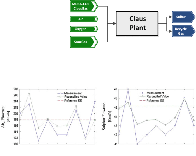
The results obtained are shown in Fig. 3. Molar ﬂows for two streams

are shown along the considered stationary point and the noisy measurements.

Reconciled ﬂowrates show lower discrepancies compared with the stationary

value.

3.2.2 Case B: DR Used for Parameter Estimation in a Coal Gasiﬁcation

Reactor

The considered gasiﬁcation process is a pressurised entrained ﬂow gasiﬁcation

reactor, as described in chapter ‘‘Modelling Syngas Generation’’ , Sect. 2, but

considering it to be a kinetic reactor as described in Perez-Fortes et al. [10]. The

feed to the gasiﬁer is composed of dry raw carbon material that is fed means of

pneumatic transportation with nitrogen at high pressure. Because nonconventional

compounds are used to model this reactor, a set of reaction extensions has been

created to cope with such system and to incorporate the stoichiometry related to

Fig. 2 Considered Claus

plant scheme, for mass

streams reconciliation

Fig. 3 Reconciled total molar ﬂows for the Claus Plant

308 A. D. Bojarski et al.

the involved reactions. These extensions enable to deﬁne sets of user-deﬁned

parameters that pile up several different physical parameters to overcome the lack

of some of them. A set of nine parameters p

–p

are deﬁned in such a way that

each one includes parameters such as pre-exponential factors for each considered

reaction, average char particle size, reactor porosity (in terms of fraction of par-

ticles and gas), deﬁned ratios in the feed composition and others. Four different

main reactions are considered:

• CHAR þO

! Reaction products:

• CHAR þH

O ! Reaction products:

• CHAR þH

! Reaction products:

• CHAR þCO

! Reaction products:

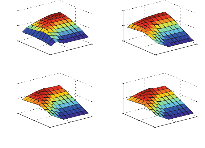
As a ﬁrst step, a sensibility analysis of the output molar fractions to the different

parameters is carried out to estimate which are the most inﬂuential set of

parameters. Figure 4 shows the effect of the parameters p

and p

at different levels

and for different combinations of the remaining ones in the fraction H

in the outlet

stream. Only two different behaviours can be noticed from the curves in Fig. 4.

The ﬁrst one is in the upper-left corner that corresponds to low levels of parameter

that is related to the pre-exponential factor of the CHAR ? H

reaction. The

remaining three surfaces show a very similar behaviour among them, and only

slight differences can be noticed at higher p

values.

0.2

0.4

Level

fraction

0.2

0.4

Level

fraction

0.2

0.4

Level

fraction

0.2

0.4

Level

fraction

Fig. 4 H

fraction parametric dependence at different levels of parameters p3-p9

Industrial Data Collection 309

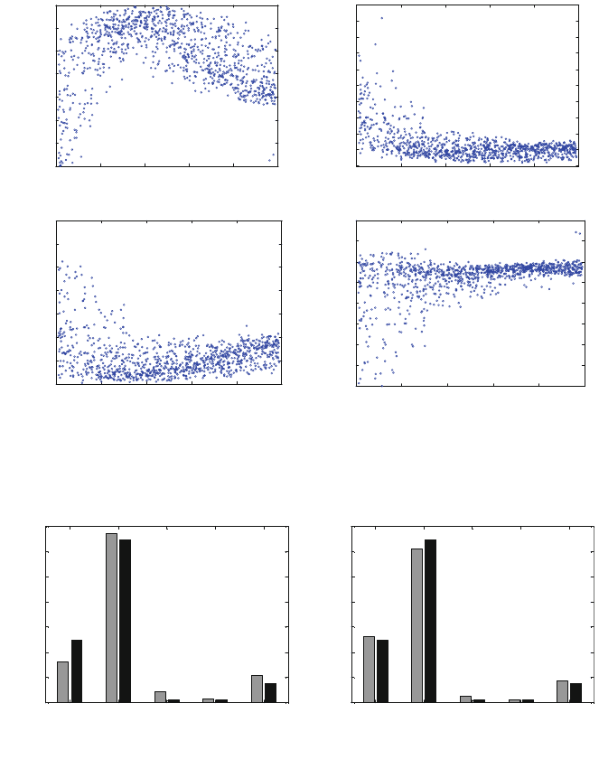
Other sensitivity analysis studied the effect on H

,CO

, CO and N

fractions

against p

at different levels in the remaining parameters. It can be seen that the

system behaviour regarding parameter p

is highly nonlinear for some of the

variables but no so much for others, see Fig. 5.

Two different raw material compositions and their corresponding output

composition are used as variables to be reconciled by solving the DR and

parameter estimation problem. Figure 6 shows the results obtained showing lower

0 20 40 60 80 100

0.05

0.1

0.15

0.2

0.25

0.3

0.35

parameter p

level

fraction

0 20 40 60 80 100

0.05

0.1

0.15

0.2

0.25

0.3

0.35

0.4

0.45

0.5

0.55

parameter p

level

fraction

0 20 40 60 80 100

0.1

0.2

0.3

0.4

0.5

0.6

0.7

parameter p

level

fraction

0 20 40 60 80 100

0.1

0.2

0.3

0.4

0.5

0.6

0.7

0.8

parameter p

level

CO fraction

Fig. 5 H2, CO2, CO and N2 fractions against p1 for different values of the remaining

H2 CO CO2 H2S H2

0.1

0.2

0.3

0.4

0.5

0.6

0.7

Molar Fraction

H2 CO CO2 H2S H2

0.1

0.2

0.3

0.4

0.5

0.6

0.7

Molar Fraction

Fig. 6 H2, CO, CO2 and N2 reactor efﬂuent molar fractions. Left side before parameters adjust,

right side: after parameters adjust

310 A. D. Bojarski et al.

discrepancies in the model results when the parameter estimation is performed,

see specially the H

fraction.

The ﬁrst example showed how different input variables relationship should be

changed to produce a lower noise in the model predictions, whereas the second

example showed how different model parameters can be tuned to improve the

model-predicting capabilities. In both examples, DR has been used to improve the

quality of data, so patterns and trends can be identiﬁed with ease.

4 Data Mining

The former section used historical data to improve the reliability of model pre-

dictions by estimating model parameters or by modifying the possible input

variables values. Many other different points of view, which do not rely on a model

to extract information, are available; and they are broadly known as data-mining

techniques.

Data mining has recently emerged as a new ﬁeld whose main objectives are

developing and reﬁning concepts and tools that may sometimes have been

developed in other disciplines to provide the user of data bases with powerful tools

to transform data into useful knowledge [1, 11].

Knowledge is one of the most valuable assets in almost any human activity.

In business, for example, having a good command of all the related issues

(purchasing, marketing, design, production, maintenance and distribution) enables

a company to differentiate itself from competitors and to compete efﬁciently and

effectively to the best of its ability.

There are many possible deﬁnitions of data mining but a very simple and

accurate one is given by Han and Kamber [12]: ‘Simply stated, data mining refers

to extracting or ‘‘mining’’ knowledge from large amounts of data’. In this deﬁ-

nition, the existing difference between data and knowledge is clearly highlighted.

4.1 Statistical Process Control

During the recent years, many research works have been devoted to the devel-

opment and improvement of a set of statistical tools that enable the process

operator to determine whether the process is working as expected. Online process

performance monitoring and product quality prediction in real time ensure safe

and proﬁtable operation because they provide the opportunity to take corrective

actions before the effects of excursions from normal operation ruin compromise

plant operation.

Common operation policies includemonitoringjusta few processvariables thatare

thought as critical variables and whose operation window is usually well deﬁned

between an upper and a lower bound. Although this is a common industrial practice,

Industrial Data Collection 311

it was extensively demonstrated that it is not an efﬁcient and consistent approach

when it comes to determining whether the process is or not in control.

Process state is commonly determined by multivariate observation vectors, and

therefore, a consistent approach, which considers the multivariate nature of the

system, has to be applied to classify the process state. The importance of con-

sidering a vector of variables as a whole instead of a set of independent mea-

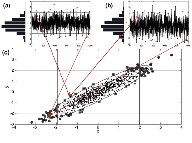
surements is easy to understand considering the simple case showed in Fig. 7.

Let us consider the case of two normal distributed variables that are simulta-

neously measured in a process (see Fig. 7a, b). Two particular observation vectors

are highlighted in Fig. 7a and b. First, let us analyze point A. This observation

would have been considered as ‘in control’ observations if the two charts (a) and

(b) were considered to monitor the process because it falls in the conﬁdence region

for a given signiﬁcance level (a). On the other hand, when the bivariate nature

of the process is taken into account, see Fig. 7c, it ﬁres an ‘out of control alarm’.

The opposite situation happens to point B. In this case, this point ﬁres an ‘out of

control alarm’ for the separate charts but behaves as ‘in control point’ in the

bivariate case. The case shown in Fig. 7 is a classic example used to reveal the

importance of considering multivariate processes as such, instead of simply

neglecting the relationships among variables [1, 13].

The knowledge of the former kind of behaviour has attracted the interest of

many research groups that have conducted extensive works intended to ﬁnd

effective methodologies to deal with this problem. However, considering the

Fig. 7 Differences between univariate and multivariate control charts

312 A. D. Bojarski et al.

multivariate nature of an industrial process is not a trivial task. Working with many

variables could make the monitoring-related tasks much more complicated.

During recent years, many successful applications of multivariate statistical

process control (MSPC) have been presented for monitoring and fault diagnosis

purposes in the case of continuous and batch processes. A common industrial

practice is to monitor the batch progress by exploiting the information contained in

a historical database of successful batches using projection techniques, such as

principal components analysis (PCA), partial least squares (PLS) and independent

component analysis (ICA).

Most of the former techniques allow for estimating the normal operating con-

dition (NOC). The knowledge of such condition enables both to develop an

empirical model of the process in terms of latent variables and to calculate sta-

tistical conﬁdence limits that will be used to test the progress of new batches; both

tasks are preformed ofﬂine. Once the model is set for online monitoring, new

process observations are analyzed to decide whether the process is under control.

Each new observation is projected into the reduced space deﬁned by the latent

variables, and the corresponding statistics is calculated and compared against their

critical values. Among the former-mentioned techniques, we focus on PCA, given

its broad use and its ease of implementation.

4.2 PCA-Based Techniques Applied for ‘Data Mining’

The PCA-based approach for monitoring and fault diagnosis purposes is one of the

most popular methods when predictions of not measured variables are not needed.

The basic concepts and schemes to implement a PCA-based monitoring strategy

are explained along this section. It is the reader’s duty to ﬁnd and deal with the

particularities related to the adaptation of this strategy to some alternative

schemes, such as moving windows, exponential weighting or dynamic-PCA.

Originally, the main application of PCA was related to exploratory data analysis

because of its ability to compress the meaningful information in a few dimensions

usually enabling a graphic analysis of the data behaviour. It was this compression

and reduction capability that reinforced the interest of many researchers in using

PCA-based approaches to overcome some of the main problems observed when

implementing monitoring schemes in the original (measurement) space. In this

sense, PCA-based approaches are specially suited for recognising if a given pattern

is present in a set of data.

4.2.1 Principal Components Analysis: Basics

PCA is just one of several latent variables projection techniques. From the mathe-

matical point of view, obtaining the principal directions is merely a space pro-

jection problem in which the projection space fulﬁls some special requirements.

Industrial Data Collection 313

The principal component space is an ‘ordered space’ in which each direction is

hierarchically ordered in terms of its variance. In addition, principal directions are

requested to be orthogonal. The principal components directions come as a solution

of optimization problem in which it is desired to ﬁnd a set of orthogonal vectors that

maximize the data variance along them. The solution of this problem can be ana-

lytically obtained [13] by performing a singular value decomposition of the system

covariance matrix (R), as in Eq. 6.

R ¼



; ð6Þ

where



K is the eigenvalues diagonal matrix and



P is the corresponding eigen-

vectors matrix. The columns of



P deﬁne the principal component directions. They

are arranged in descending order in terms of variance that is given by the corre-

sponding eigenvalue [13]. There are many efﬁcient algorithms that can be applied

to calculate



K, also known as loading vectors matrix. One of the most popular is

the NIPALS algorithm presented by Wold [14]. Once the loading vector matrix

has been calculated, the data matrix can be rewritten as in Eq. 7.

X ¼



; ð7Þ

where



T is the scores matrix that contains the coordinates of matrix of X in the

latent space.

Usually, the actual covariance matrix (R) is unknown and the sample covari-

ance matrix (S) is used instead. An important result that the reader should always

consider is that, as it was mentioned before, S is to X as



K is to



S ¼

ðI  1Þ

X ¼



ð8Þ



K ¼

ðI  1Þ



T ¼ diag k

; k

; k

½



; 8 j ¼ 1; 2; ...; J ð9Þ

It is clear from Eq. 9 that principal components are essentially uncorrelated

because



K is a diagonal matrix.

As it was mentioned before, the most useful property of PCA is its capacity to

condense most of data variability in just a few ﬁrst directions. As a consequence,

it is possible to represent the data using just a few directions without losing much

of the meaningful information in data. PCA-based monitoring strategies exploit

this property to reduce the original space from R

to R

(with R \ J) splitting the

original space in two well-differenced domains, the ﬁrst is referred as the retained

space (R

) and the second as the excluded space (R

JR

). According to this, the

loading and score matrices can be reordered as in Eqs. 10 and 11.



P ¼ P



ð10Þ



T ¼ T



; ð11Þ

314 A. D. Bojarski et al.

where



P 2 R

JJ

is the loading matrix used when considering the whole latent

space, P 2 R

JR

is the loading matrix for the retained space and

P 2 R

JðJRÞ

contains the excluded principal directions. Similarly,



T 2 R

IJ

deﬁnes the

coordinates of X in the full principal components space. Finally, T 2 R

IR

and

T 2 R

IðJRÞ

are the coordinates of X in the retained and excluded space,

respectively. Reordering Eq. 7, we obtain:

X ¼



¼ TP

: ð12Þ

In literature, it is usually found that T ¼ XP, and therefore,

X and E result:

X ¼ XPP

ð13Þ

E ¼ XI PP



; ð14Þ

where E, is the residuals matrix that is generated by the exclusion of the principal

directions contained in

One central point when using projection-based techniques is the goodness of the

representation in the reduced space. This point is closely related to the minimum

number of directions that have to be used to achieve a reasonable data description

in the PC’s space. One characteristic parameter in multivariate statistics is the total

variance of the data (r

¼ trðRÞ ). Equation 15 shows how to estimate r

in both

the original and the PC’s spaces:

¼ trðRÞ¼

j¼1

: ð15Þ

It is easy to note from Eq. 15 that each principal direction explains just a

fraction of r

, the percentage explained by the rth component is:

%; T

 100; 8 r ¼ 1; 2; ::; J: ð16Þ

The percentage of the total variance explained in the R-dimensional space (PC’s

1toR) is:

r¼1:R

%; T

r¼1



100

: ð17Þ

It is also possible to estimate the fraction of the variance of a particular variable

in the R-dimensional by using Eq. 18.

r¼1:R

r¼1

j; r

j; j

: ð18Þ

Industrial Data Collection 315

There exist many ways to determine the number of principal components to be

retained (R). Many of these are closely related to the afore-mentioned goodness-

related indexes. The most simple may result the cumulative percent variance

(CPV) criteria in which one should retain as many PC’s as needed to match a

previously deﬁned percentage of reconstruction for r

. Further information

regarding this and other criteria can be found elsewhere [13, 15].

4.3 PCA-Based Monitoring Scheme

The set up of a statistical process monitoring scheme is usually presented as a

two-stage procedure. Stage I, also referred as ‘off line stage’, includes the main

calculations to build the PCA model and to estimate the threshold values for the

hypothesis testing. Although it is not frequently mentioned, a central step is the

correct pretreatment of the data set that will be used to calculate the model.

Pretreatment activities may include—but are not limited to—measurement

scaling, outlier detection and data clustering and classiﬁcation. Data pretreatment

is not usually covered in research papers dealing with process monitoring;

nevertheless, the success of the whole monitoring strategy strongly depends on it.

Pretreatment-related activities by itself do constitute a whole subject, and are out

of the scope of this chapter. Descriptions of the most commonly used tools for data

pretreatment, its purposes and limitations can be found elsewhere [13]. The main

objective of data pretreatment is to obtain a data set that can be considered as a

good sample of the process operation in normal operation condition (NOC)

because they will be used to build the PCA model and to determine the normal

region.

Let us consider X to be the process data matrix after an appropriate pretreat-

ment. As it is usually the case, process observations are made of various measured

variables with different measurement units and variability ranges. As a conse-

quence, a very common step during stage I is variable scaling or standardization.

This procedure results useful for both putting measurements a common unit-less

scale and avoiding undesired side effects that can arise from working with vari-

ables in very different scales and ranges. Once X has been properly scaled, the

PCA model is calculated as it is explained in previous chapter ‘‘Modelling Syngas

Generation’’ i n Sect. 2.1, and the normal operation regions have to be determined.

The former PCA model serves as basis for comparison of new metrics, con-

sequently, the adequacy of these approaches heavily depends on how well this

PCA model represents the plant behaviour.

It is a very common practice in PCA-based monitoring approaches to use two

complementary statistics to follow the process evolution. Typical statistic metrics

are the Hotelling’s T

[16] and the squared prediction error (SPE).

The T

statistic metric is widely employed in multivariate systems analysis, and

it was proposed as a generalisation of Student’s t distribution to the multivariate

case. It is based on the Mahalanobis distance, which confers it the capacity for

316 A. D. Bojarski et al.

evaluating changes in the system’s correlation structure and to decide if one

observation can be considered part of a given data population. Consequently, it is

useful for devising if observed process deviations can or cannot be considered

within the normal process variability. The T

for a given observation vector

2 R

can be calculated as in Eq. 19.

¼ x







1







; ð19Þ

where



x is the population mean and matrix S is its covariance.

The SPE-statistics, (referred as Q-statistic in some cases), is deﬁned as the

summation of the squared errors between the original signal and the reconstructed

signal using the retained PCs, see Eq. 20.

SPE

¼ e

¼ I PP





: ð20Þ

SPE-statistics accounts for the distance between the measured observation

point and its projection into the reduced PCA space. If the SPE value exceeds

the threshold values for a given process realization, the last is said to show a

completely new behaviour not shown by the data in the NOC. Threshold values

for both statistics strongly depend on the assumptions and simpliﬁcations that

the analyst makes. Detailed procedures for the calculation of the control limit

values can be found in literature see, for example, Nomikos and MacGregor

[17].

Stage II of the PCA-based monitoring is the actual use of the PCA model on the

plant current operating conditions and analyses its possible discrepancies com-

pared with the NOC calculated on stage I. In this sense, new data points (x

) allow

for calculating the new values for T

and SPE. These values are compared against

the respective control limit values T

lim

and SPE

lim



such that the following

inequalities hold.

lim

ð21Þ

SPE

\SPE

lim

: ð22Þ

If some or both of the former inequalities do not hold (for a certain number of

consecutive observations), then, the system is said to be out of normal operation

conditions. These comparisons are typically done using monitoring-control charts

where the T

and SPE values are plotted together with the control limit values.

Latent projections, projection residuals, T

and SPE values for each new obser-

vation are calculated as follows:

¼ P

ð23Þ

¼ t

1

ð24Þ

¼ I PP



ð25Þ

Industrial Data Collection 317

Puigjaner L. (ed.) Syngas from Waste - Emerging Technologies

Подождите немного. Документ загружается.