Poto?nik P. (Ed.) Natural Gas
Подождите немного. Документ загружается.

Natural gas properties and ow computation 511
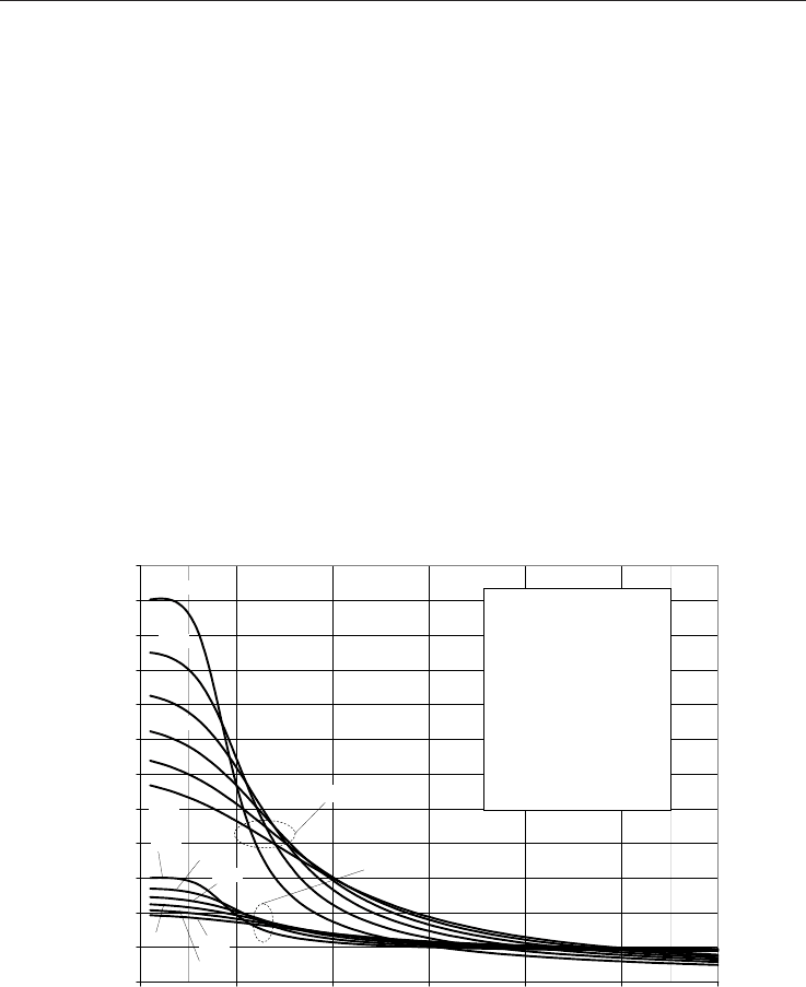
Table 2 depicts the calculation procedure. Prior to the calculation of the molar heat
capacities, isentropic exponent and JT coefficient, the density and the compression factor of
a natural gas must be calculated. The false position method is combined with the successive
bisection method to calculate the roots of the equation of state [Starling & Savidge, 1992].
Table 2. The input/output parameters and the procedure for the computation of the natural
gas properties.
Input parameters – constant:
molar gas constant (R=8314.51 J/(kmol·K))
natural gas equation of state parameters (a
n
, b
n
, c
n
, k
n
, u
n
, g
n
, q
n
, f
n
, s
n
, w
n
; n=1, 2,...,58),
characterization parameters (M
i
, E
i
, K
i
, G
i
, Q
i
, F
i
, S
i
, W
i
; i=1,...,21) and binary interaction
parameters (
*
, ji
E ,
ji
U
,
,
ji
K
,
,
*
, ji
G ) (see ISO 12213-2)
DIPPR/AIChE gas heat capacity constants (a
j
, b
j
, c
j
, d
j
;, e
j
; j=1,2,...,N)
Input parameters – time varying:
absolute pressure: p [MPa]
absolute temperature: T [K]
molar fractions of the natural gas mixture: y
i
; i=1,2,...,N
Calculation procedure:
1. mixture size parameter
K
(Eq. 13), second virial coefficient
B
(Eq. 14) and temperature
dependent coefficients
*
n
C (Eq. 18)
2. compression factor
Z
(Eq. 8) (see ISO-12213-2 for details of calculation)
3. molar density
RTZp
m
/
, density
m
M
, reduced density
mr
K
3
and
molar volume
mm
v
/1
.
4. coefficients
n
D and
n
D
1
(Eqs. 32 and 36)
5. 1
st
and 2
nd
derivative of the second virial coefficient B: B
(Eq. 23) and B
(Eq. 24)
6. 1
st
and 2
nd
derivative of the coefficient
*
n
C :
*
n
C (Eq. 25) and
*
n
C (Eq. 26)
7. 1
st
derivative of the compression factor Z:
p
TZ
(Eq. 33)
8. partial derivatives of pressure:
m
v
Tp
(Eq. 29) and
T
m
vp
(Eq. 38)
9. ideal molar heat capacity of a gas mixture at constant pressure:
pIm
c
,
(Eq. 27)
10. molar heat capacity of a gas mixture at constant volume:
vm
c
,
(Eqs. 9)
11. molar heat capacity of a gas mixture at constant pressure:
pm
c
,
(Eqs. 4)
12. isentropic exponent
(Eq. 37)
13. Joule-Thomson coefficient
JT
(Eq. 39)
4. Comparison with experimental results
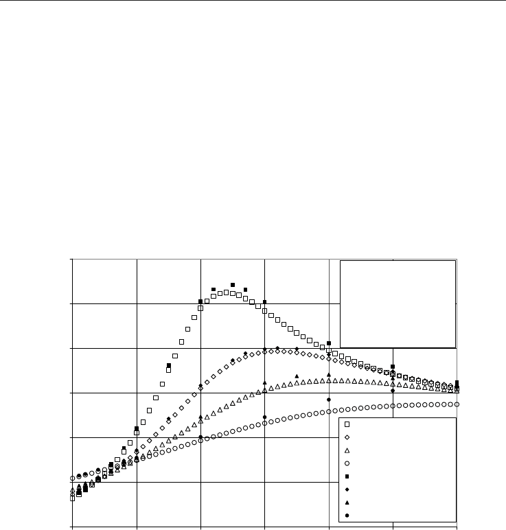
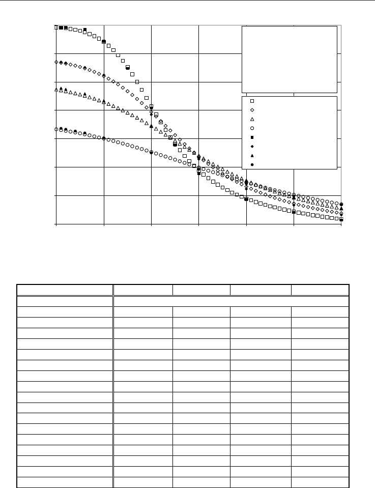
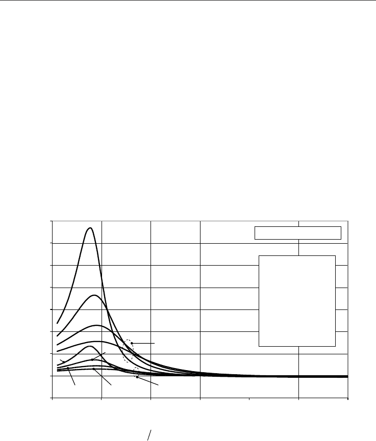
In order to compare the calculation results, for the specific heat capacity
p
c and the JT
coefficient
JT
, with the corresponding high accuracy measurement data (Ernst et al., 2001),
we assume the identical artificial natural gas mixture with the following mole fractions:
x
CH4
=0.79942, x
C2H6
=0.05029, x
C3H8
=0.03000, x
CO2
=0.02090 and x
N2
=0.09939. The results of the
measurements (Ernst et al., 2001) and the results of the calculation of the specific heat
capacity
p
c
and the JT coefficient
JT
of the natural gas mixture, for absolute pressure
ranging from 0 MPa to 30 MPa in 0.5 MPa steps and for four upstream temperatures (250 K,
275 K, 300 K and 350 K), are shown in Fig. 2 and 3, respectively. The differences between the
calculated values and the corresponding measurement results (Ernst et al., 2001), for the
p
c
and
JT
, are shown in Table 3 and 4, respectively.
1.50
2.00
2.50
3.00
3.50
4.00
4.50
0 5 10 15 20 25 30
Pressure [MPa]
c
p
- specific heat capacity [J/(g*K)]
Calculated at 250 K
Calculated at 275 K
Calculated at 300 K
Calculated at 350 K
Measured at 250 K, Ernst et al.
Measured at 275 K, Ernst et al.
Measured at 300 K, Ernst et al.
Measured at 350 K, Ernst et al.
Natural gas analysis
(mole fractions):
m
ethane.........0.79942
ethane..........0.05029
propane.........0.03000
carbon dioxide..0.02090
nitrogen........0.09939
Fig. 2. Calculated and measured molar heat capacity at constant pressure of the natural gas
mixture.
From Table 3 it can be seen that the calculated values of
p
c are within ±0.08 J/(g*K) with the
measurement results for the pressures up to 12 MPa. At higher pressures, up to 30 MPa, the
difference increases but never exceeds ±0.2 J/(g*K). For pressures up to 12 MPa the relative
difference between the calculated and experimentally obtained
p
c never exceeds ±2.00%.
Natural Gas512
0.00
1.00
2.00
3.00
4.00
5.00
6.00
7.00
0 5 10 15 20 25 30
Pressure [MPa]
μ
JT
- Joule-Thomson coefficient [K/MPa]
Calculated at 250 K
Calculated at 275 K
Calculated at 300 K
Calculated at 350K
Measured at 250 K, Ernst et al.
Measured at 275 K, Ernst et al.
Measured at 300 K, Ernst et al.
Measured at 350 K, Ernst et al.
Natural gas analysis
(mole fractions):
m
ethane.........0.79942
ethane..........0.05029
propane.........0.03000
carbon dioxide..0.02090
nitrogen........0.09939
Fig. 3. Calculated and measured JT coefficient of the natural gas mixture.
P [MPa]: T [K]
250 275 300 350
(c
p_calculated
- c
p_measured
) [J/(g*K)]
0.5
-0.015 -0.018 -0.018 -0.012
1.0
-0.002 -0.014 -0.016 -0.011
2.0 -0.012 -0.019 -0.022 -0.020
3.0
-0.032 -0.020 -0.023 -0.026
4.0 -0.041 -0.023 -0.021 -0.027
5.0
-0.051 -0.022 -0.025 -0.029
7.5
-0.055 -0.032 - -
10.0
-0.077 -0.033 -0.048 -0.042
11.0
-0.075 - - -
12.5
-0.092 -0.030 - -
13.5
-0.097 -0.039 - -
15.0 -0.098 -0.033 -0.082 -0.069
16.0
- -0.036 - -
17.5 - -0.043 -0.075 -
20.0
-0.081 -0.048 -0.066 -0.134
25.0
-0.082 -0.033 -0.064 -0.171
30.0
-0.077 -0.025 -0.070 -0.194
Table 3. Difference between the calculated and measured specific heat capacity at constant
pressure of a natural gas.
P [MPa]: T [K] 250 275 300 350
(μ
JT_calculated
- μ
JT_measured
) [K/MPa]
0.5
-0.014 -0.023 -0.075 -0.059
1.0
-0.032 -0.024 -0.068 -0.053
2.0
- - - -0.051
3.0
-0.092 -0.032 -0.069 -0.049
5.0
-0.022 -0.036 -0.044 -0.026
7.5
0.043 - - -
10.0
0.060 0.096 0.019 0.030
12.5
0.034 - - -
15.0
0.113 0.093 0.050 0.061
20.0
0.029 0.084 0.009 0.047
25.0
0.025 0.059 0.002 0.043
30.0
0.031 0.052 0.005 0.012
Table 4. Difference between the calculated and measured JT coefficient of a natural gas.
1.00
2.00
3.00
4.00
5.00
6.00
0 5 10 15 20 25 30
Pressure [MPa]
κ
- isentropic exponent
Natural gas analysis
(mole fractions):
methane.........0.79942
ethane..........0.05029
propane.........0.03000
carbon dioxide..0.02090
nitrogen........0.09939
250 K
275 K
300 K
350 K
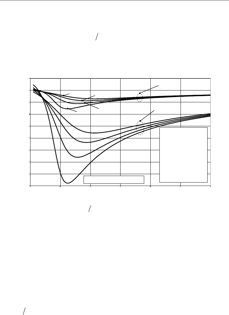
Fig. 4. Calculated isentropic exponent of the natural gas mixture.
From Table 4 it can be seen that the calculated values of
JT
are within ±0.113 K/MPa with
the experimental results for the pressures up to 30 MPa. The relative difference increases
with the increase of pressure but never exceeds ±2.5% for the pressures up to 12 MPa. At
higher pressures, when the values of
JT
are close to zero, the relative difference may
increase significantly. The calculation results obtained for pure methane and methane-
ethane mixture are in considerably better agreement with the corresponding experimental
data (Ernst et al., 2001) than for the natural gas mixture shown above. We estimate that the
relative uncertainty of the calculated
p
c and
JT
of the AGA-8 natural gas mixtures in
common industrial operating conditions (pressure range 0-12 MPa and temperature range
Natural gas properties and ow computation 513
0.00
1.00
2.00
3.00
4.00
5.00
6.00
7.00
0 5 10 15 20 25 30
Pressure [MPa]
μ
JT
- Joule-Thomson coefficient [K/MPa]
Calculated at 250 K
Calculated at 275 K
Calculated at 300 K
Calculated at 350K
Measured at 250 K, Ernst et al.
Measured at 275 K, Ernst et al.
Measured at 300 K, Ernst et al.
Measured at 350 K, Ernst et al.
Natural gas analysis
(mole fractions):
m
ethane.........0.79942
ethane..........0.05029
propane.........0.03000
carbon dioxide..0.02090
nitrogen........0.09939
Fig. 3. Calculated and measured JT coefficient of the natural gas mixture.
P [MPa]: T [K]
250 275 300 350
(c
p_calculated
- c
p_measured
) [J/(g*K)]
0.5
-0.015 -0.018 -0.018 -0.012
1.0
-0.002 -0.014 -0.016 -0.011
2.0
-0.012 -0.019 -0.022 -0.020
3.0
-0.032 -0.020 -0.023 -0.026
4.0
-0.041 -0.023 -0.021 -0.027
5.0
-0.051 -0.022 -0.025 -0.029
7.5
-0.055 -0.032 - -
10.0
-0.077 -0.033 -0.048 -0.042
11.0
-0.075 - - -
12.5
-0.092 -0.030 - -
13.5
-0.097 -0.039 - -
15.0
-0.098 -0.033 -0.082 -0.069
16.0
- -0.036 - -
17.5
- -0.043 -0.075 -
20.0
-0.081 -0.048 -0.066 -0.134
25.0
-0.082 -0.033 -0.064 -0.171
30.0
-0.077 -0.025 -0.070 -0.194
Table 3. Difference between the calculated and measured specific heat capacity at constant
pressure of a natural gas.
P [MPa]: T [K] 250 275 300 350
(μ
JT_calculated
- μ
JT_measured
) [K/MPa]
0.5
-0.014 -0.023 -0.075 -0.059
1.0 -0.032 -0.024 -0.068 -0.053
2.0
- - - -0.051
3.0
-0.092 -0.032 -0.069 -0.049
5.0
-0.022 -0.036 -0.044 -0.026
7.5
0.043 - - -
10.0
0.060 0.096 0.019 0.030
12.5
0.034 - - -
15.0 0.113 0.093 0.050 0.061
20.0
0.029 0.084 0.009 0.047
25.0 0.025 0.059 0.002 0.043
30.0
0.031 0.052 0.005 0.012
Table 4. Difference between the calculated and measured JT coefficient of a natural gas.
1.00
2.00
3.00
4.00
5.00
6.00
0 5 10 15 20 25 30
Pressure [MPa]
κ
- isentropic exponent
Natural gas analysis
(mole fractions):
methane.........0.79942
ethane..........0.05029
propane.........0.03000
carbon dioxide..0.02090
nitrogen........0.09939
250 K
275 K
300 K
350 K
Fig. 4. Calculated isentropic exponent of the natural gas mixture.
From Table 4 it can be seen that the calculated values of
JT
are within ±0.113 K/MPa with
the experimental results for the pressures up to 30 MPa. The relative difference increases
with the increase of pressure but never exceeds ±2.5% for the pressures up to 12 MPa. At
higher pressures, when the values of
JT
are close to zero, the relative difference may
increase significantly. The calculation results obtained for pure methane and methane-
ethane mixture are in considerably better agreement with the corresponding experimental
data (Ernst et al., 2001) than for the natural gas mixture shown above. We estimate that the
relative uncertainty of the calculated
p
c and
JT
of the AGA-8 natural gas mixtures in
common industrial operating conditions (pressure range 0-12 MPa and temperature range
Natural Gas514
250-350 K) is unlikely to exceed ±3.00 % and ±4.00 %, respectively. Fig. 4 shows the results of
the calculation of the isentropic exponent. Since the isentropic exponent is a theoretical
parameter there exist no experimental data for its verification.
5. Flow rate measurement
Flow rate equations for differential pressure meters assume a constant fluid density of a
fluid within the meter. This assumption applies only to incompressible flows. In the case of
compressible flows, a correction must be made. This correction is known as adiabatic
expansion factor, which depends on several parameters including differential pressure,
absolute pressure, pipe inside diameter, differential device bore diameter and isentropic
exponent. Isentropic exponent has a limited effect on the adiabatic correction factor but has
to be calculated if accurate flow rate measurements are needed.
Flow direction
Natural gas
Orifice plate
p
u
, T
u
p
d
, T
d
p
D
D
6D
d
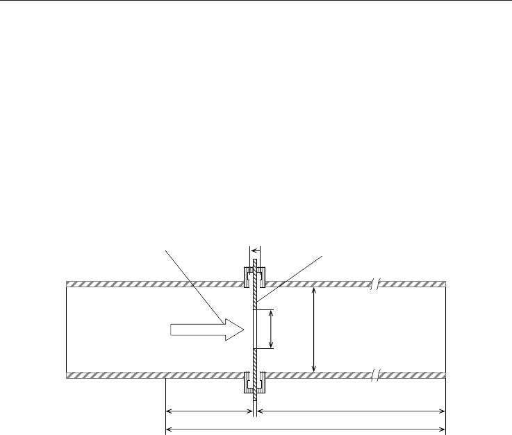
Fig. 5. The schematic diagram of the natural gas flow rate measurement using an orifice
plate with corner taps.
When a gas expands through the restriction to a lower pressure it changes its temperature
and density (Fig. 5). This process occurs under the conditions of constant enthalpy and is
known as JT expansion (Shoemaker at al., 1996). It can also be considered as an adiabatic
effect because the pressure change occurs too quickly for significant heat transfer to take
place. The temperature change is related to pressure change and is characterized by the JT
coefficient. The temperature change increases with the increase of the pressure drop and is
proportional with the JT coefficient. According to (ISO5167, 2003) the upstream temperature
is used for the calculation of flow rate but the temperature is preferably measured
downstream of the differential device. The use of downstream instead of upstream
temperature may cause a flow rate measurement error due to the difference in the gas
density caused by the temperature change. Our objective is to derive the numerical
procedure for the calculation of the natural gas specific heat capacity, isentropic exponent
and JT coefficient that can be used for the compensation of flow rate error. In order to make
the computationally intensive compensation procedure applicable to low computing power
real-time measurement systems the low complexity surrogate models of original procedures
will be derived using the computational intelligence methods: ANN and GMDH. The
surrogate models have to be tailored to meet the constraints imposed on the approximation
accuracy and the complexity of the model, i.e. the execution time (ET).
6. Compensation of flow rate error
We investigated the combined effect of the JT coefficient and the isentropic exponent of a
natural gas on the accuracy of flow rate measurements based on differential devices. The
measurement of a natural gas (ISO-12213-2, 2006) flowing in a pipeline through orifice plate
with corner taps (Fig. 5) is assumed to be completely in accordance with the international
standard (ISO-5167, 2003). The detailed description of the flow rate equation with the
corresponding iterative computation scheme is given in (ISO-5167, 2003). The calculation of
the natural gas flow rate depends on multiple parameters:
dDpTPqq
uuuuuu
,,,,,,,
,
(40)
where q
u
,
u
,
u
and
u
represent the corresponding mass flowrate, density, viscosity and the
isentropic exponent calculated at upstream pressure P
u
and temperature T
u
, while D and d
denote the internal diameters of the pipe and the orifice, respectively. In case of the
upstream pressure and the downstream temperature measurement, as suggested by (ISO-
5167, 2003), the flow rate equation, Eq. (40), changes to:
dDpTPqq
ddddud
,,,,,,,
,
(41)
where q
d
,
d
,
d
and
d
denote the corresponding mass flow rate, density, viscosity and the
isentropic exponent calculated in “downstream conditions” i.e. at the upstream pressure p
u
and the downstream temperature T
d
. For certain natural gas compositions and operating
conditions the flow rate q
d
may differ significantly from q
u
and the corresponding
compensation for the temperature drop effects, due to JT expansion, may be necessary in
order to preserve the requested measurement accuracy (Maric & Ivek, 2010).
The flow rate correction factor K can be obtained by dividing the true flow rate q
u
calculated
in the upstream conditions, Eq. (40), by the flow rate q
d
calculated in the “downstream
conditions”, Eq. (41):
d
u
q
q
K
(42)
For the given correction factor Eq. (42), the flow rate at the upstream pressure and
temperature can be calculated directly from the flow rate computed in the “downstream
conditions”, i.e.
du
qKq . Our objective is to derive the GMDH polynomial model of the
flow rate correction factor. Given the surrogate model (K
SM
) for the flow rate correction
factor Eq. (42), the true flow rate q
u
can be approximated by:
dSMSM
qKq
, where q
SM
denotes the corrected flow rate.
The flow rate through orifice is proportional to the expansibility factor ε, which is related to
the isentropic exponent κ (ISO-5167, 2003):

Natural gas properties and ow computation 515
250-350 K) is unlikely to exceed ±3.00 % and ±4.00 %, respectively. Fig. 4 shows the results of
the calculation of the isentropic exponent. Since the isentropic exponent is a theoretical
parameter there exist no experimental data for its verification.
5. Flow rate measurement
Flow rate equations for differential pressure meters assume a constant fluid density of a
fluid within the meter. This assumption applies only to incompressible flows. In the case of
compressible flows, a correction must be made. This correction is known as adiabatic
expansion factor, which depends on several parameters including differential pressure,
absolute pressure, pipe inside diameter, differential device bore diameter and isentropic
exponent. Isentropic exponent has a limited effect on the adiabatic correction factor but has
to be calculated if accurate flow rate measurements are needed.
Flow direction
Natural gas
Orifice plate
p
u
, T
u
p
d
, T
d
p
D
D
6D
d
Fig. 5. The schematic diagram of the natural gas flow rate measurement using an orifice
plate with corner taps.
When a gas expands through the restriction to a lower pressure it changes its temperature
and density (Fig. 5). This process occurs under the conditions of constant enthalpy and is
known as JT expansion (Shoemaker at al., 1996). It can also be considered as an adiabatic
effect because the pressure change occurs too quickly for significant heat transfer to take
place. The temperature change is related to pressure change and is characterized by the JT
coefficient. The temperature change increases with the increase of the pressure drop and is
proportional with the JT coefficient. According to (ISO5167, 2003) the upstream temperature
is used for the calculation of flow rate but the temperature is preferably measured
downstream of the differential device. The use of downstream instead of upstream
temperature may cause a flow rate measurement error due to the difference in the gas
density caused by the temperature change. Our objective is to derive the numerical
procedure for the calculation of the natural gas specific heat capacity, isentropic exponent
and JT coefficient that can be used for the compensation of flow rate error. In order to make
the computationally intensive compensation procedure applicable to low computing power
real-time measurement systems the low complexity surrogate models of original procedures
will be derived using the computational intelligence methods: ANN and GMDH. The
surrogate models have to be tailored to meet the constraints imposed on the approximation
accuracy and the complexity of the model, i.e. the execution time (ET).
6. Compensation of flow rate error
We investigated the combined effect of the JT coefficient and the isentropic exponent of a
natural gas on the accuracy of flow rate measurements based on differential devices. The
measurement of a natural gas (ISO-12213-2, 2006) flowing in a pipeline through orifice plate
with corner taps (Fig. 5) is assumed to be completely in accordance with the international
standard (ISO-5167, 2003). The detailed description of the flow rate equation with the
corresponding iterative computation scheme is given in (ISO-5167, 2003). The calculation of
the natural gas flow rate depends on multiple parameters:
dDpTPqq
uuuuuu
,,,,,,,
,
(40)
where q
u
,
u
,
u
and
u
represent the corresponding mass flowrate, density, viscosity and the
isentropic exponent calculated at upstream pressure P
u
and temperature T
u
, while D and d
denote the internal diameters of the pipe and the orifice, respectively. In case of the
upstream pressure and the downstream temperature measurement, as suggested by (ISO-
5167, 2003), the flow rate equation, Eq. (40), changes to:
dDpTPqq
ddddud
,,,,,,,
,
(41)
where q
d
,
d
,
d
and
d
denote the corresponding mass flow rate, density, viscosity and the
isentropic exponent calculated in “downstream conditions” i.e. at the upstream pressure p
u
and the downstream temperature T
d
. For certain natural gas compositions and operating
conditions the flow rate q
d
may differ significantly from q
u
and the corresponding
compensation for the temperature drop effects, due to JT expansion, may be necessary in
order to preserve the requested measurement accuracy (Maric & Ivek, 2010).
The flow rate correction factor K can be obtained by dividing the true flow rate q
u
calculated
in the upstream conditions, Eq. (40), by the flow rate q
d
calculated in the “downstream
conditions”, Eq. (41):
d
u
q
q
K
(42)
For the given correction factor Eq. (42), the flow rate at the upstream pressure and
temperature can be calculated directly from the flow rate computed in the “downstream
conditions”, i.e.
du
qKq . Our objective is to derive the GMDH polynomial model of the
flow rate correction factor. Given the surrogate model (K
SM
) for the flow rate correction
factor Eq. (42), the true flow rate q
u
can be approximated by:
dSMSM
qKq , where q
SM
denotes the corrected flow rate.
The flow rate through orifice is proportional to the expansibility factor ε, which is related to
the isentropic exponent κ (ISO-5167, 2003):

Natural Gas516
/1
84
193.0256.0351.01
ud
pp
,
(43)
where β denotes the ratio of the diameter of the orifice to the inside diameter of the pipe,
while p
u
and p
d
are the absolute pressures upstream and downstream of the orifice plate,
respectively. The corresponding temperature change (T) of the gas for the orifice plate is
defined by
),(
duJTdu
TpTTT
,
(44)
where T
u
and T
d
indicate the corresponding temperatures upstream and downstream of the
orifice plate,
),(
duJT
Tp
is the JT coefficient at upstream pressure p
u
and downstream
temperature T
d
and
is the pressure loss across the orifice plate (Urner, 1997)
p
CC
CC
224
224
11
11
,
(45)
where C denotes the coefficient of discharge for orifice plate with corner taps (ISO-5167,
2003) and P is the pressure drop across the orifice plate. According to (ISO-5167, 2003), the
temperature of the fluid shall preferably be measured downstream of the primary device
but upstream temperature is to be used for the calculation of the flow rate. Within the limits
of application of the international standard ISO-5167 it is generally assumed that the
temperature drop across differential device can be neglected but it is also suggested to be
taken into account if higher accuracies are required. It is also assumed that the isentropic
exponent can be approximated by the ratio of the specific heat capacity at constant pressure
to the specific heat capacity at constant volume of ideal gas. These approximations may
produce a considerable measurement error. The relative flow measurement error E
r
is
estimated by comparing the approximate (q
d
) and the corrected (q
u
) mass flow rate i.e.
uudr
qqqE
(46)
Step Description
1
Calculate the natural gas properties (
d
, μ
J
T
and
d
) at p
u
, and T
d
, (Table 2).
2
Calculate the dynamic viscosity
d
at P
u
, and T
d
, using e.g. the residual viscosity equation
(Poling, 2000).
3 Calculate the mass flow rate q
d
and the discharge coefficient C at P
u
, T
d
and
Δp (ISO-5167, 2003).
4
Calculate the pressure loss Δ
, Eq. (45).
5 Calculate the upstream temperature T
u
in accordance with Eq. (44).
6
Calculate the natural gas properties (
u
and
u
) at p
u
, and T
u
, (Table 2).
7
Calculate the dynamic viscosity
u
at p
u
, and T
u
, using e.g. the residual viscosity equation
(Poling, 2000).
8 Calculate the mass flow rate q
u
at p
u
, T
u
and
Δp (ISO-5167, 2003).
Table 5. Precise correction of the flow rate based on downstream temperature measurement
and on the computation of natural gas properties.
The individual and the combined relative errors due to the approximations of the
temperature drop and the isentropic exponent can be estimated by using the Eq. (46). The
precise correction of the natural gas flow rate, based on upstream pressure and downstream
temperature measurement and on the computation of the corresponding natural gas
properties, is summarized in Table 5.
The procedure in Table 5 requires a double calculation of both the flow rate and the
properties of the natural gas. To reduce the computational burden we aim to derive a low-
complexity flow rate correction factor model that will enable direct compensation of the
flow rate error caused by the measurement of the downstream temperature. The correction
factor model has to be simple enough in order to be executable in real-time and accurate
enough to ensure the acceptable measurement accuracy.
7. Results of flow rate measurement simulations
In order to simulate a flow rate measurement error caused by the non-compensated
temperature drop, a natural gas mixture (Gas 3) from Annex C of (ISO-12213-2, 2006) is
assumed to flow through orifice plate with corner taps (ISO-5167, 2003) as illustrated in Fig.
5. Following the recommendations (ISO-5167, 2003), the absolute pressure is assumed to be
measured upstream (p
u
) and the temperature downstream (T
d
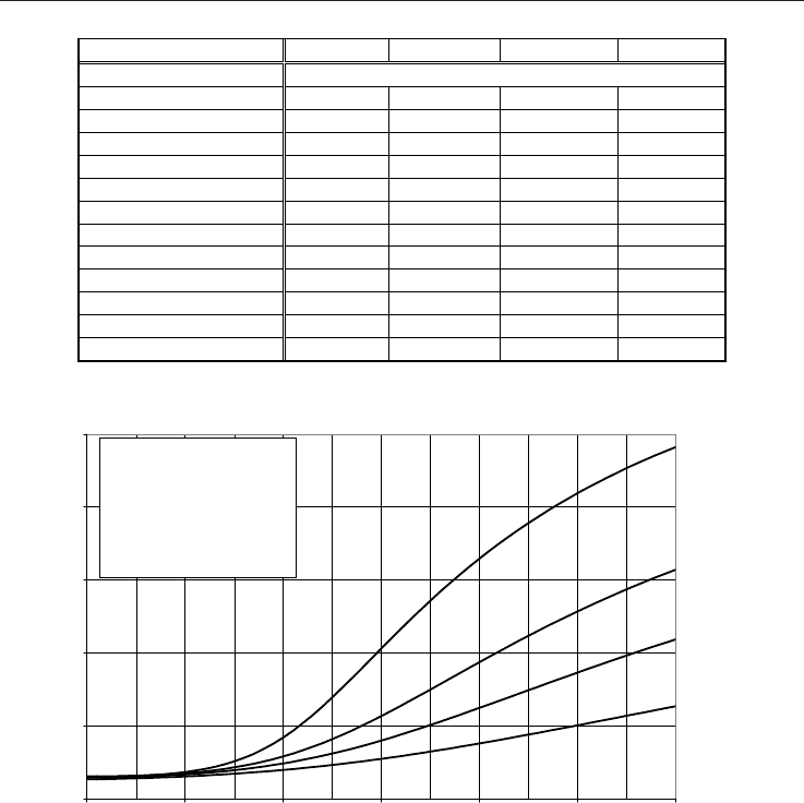
) of the primary device. Fig. 6
-0.05
0.00
0.05
0.10
0.15
0.20
0.25
0.30
0.35
0.40
0.45
0.50
0.55
0 10 20 30 40 50 60
Pressure p[MPa]
Temperature drop
T=T
1
-T
2
=
JT
[K]
245K
265K
285K
305K
325K
345K
p=100kPa
p=20kPa
245K
265K
285K
305K
325K
345K
Natural gas analysis
(mole percent):
methane.........85.90
ethane...........8.50
propane..........2.30
carbon dioxide...1.50
nitrogen.........1.00
i-butane.........0.35
n-butane.........0.35
i-pentane........0.05
n-pentane........0.05
Fig. 6. Temperature drop due to JT effect
JT
T when measuring flow rate of natural
gas mixture through orifice plate with corner taps (ISO-5167, 2003). The upstream pressure
varies from 1 MPa to 60 MPa in 1 MPa steps and upstream temperature from 245 K to 305 K
in 20 K steps for each of the two differential pressures Δp (20 kPa and 100 kPa). The internal
diameters of orifice and pipe are: d=120 mm and D=200 mm.
Natural gas properties and ow computation 517
/1
84
193.0256.0351.01
ud
pp
,
(43)
where β denotes the ratio of the diameter of the orifice to the inside diameter of the pipe,
while p
u
and p
d
are the absolute pressures upstream and downstream of the orifice plate,
respectively. The corresponding temperature change (T) of the gas for the orifice plate is
defined by
),(
duJTdu
TpTTT
,
(44)
where T
u
and T
d
indicate the corresponding temperatures upstream and downstream of the
orifice plate,
),(
duJT
Tp
is the JT coefficient at upstream pressure p
u
and downstream
temperature T
d
and
is the pressure loss across the orifice plate (Urner, 1997)
p
CC
CC
224
224
11
11
,
(45)
where C denotes the coefficient of discharge for orifice plate with corner taps (ISO-5167,
2003) and P is the pressure drop across the orifice plate. According to (ISO-5167, 2003), the
temperature of the fluid shall preferably be measured downstream of the primary device
but upstream temperature is to be used for the calculation of the flow rate. Within the limits
of application of the international standard ISO-5167 it is generally assumed that the
temperature drop across differential device can be neglected but it is also suggested to be
taken into account if higher accuracies are required. It is also assumed that the isentropic
exponent can be approximated by the ratio of the specific heat capacity at constant pressure
to the specific heat capacity at constant volume of ideal gas. These approximations may
produce a considerable measurement error. The relative flow measurement error E
r
is
estimated by comparing the approximate (q
d
) and the corrected (q
u
) mass flow rate i.e.
uudr
qqqE
(46)
Step Description
1
Calculate the natural gas properties (
d
, μ
J
T
and
d
) at p
u
, and T
d
, (Table 2).
2
Calculate the dynamic viscosity
d
at P
u
, and T
d
, using e.g. the residual viscosity equation
(Poling, 2000).
3 Calculate the mass flow rate q
d
and the discharge coefficient C at P
u
, T
d
and
Δp (ISO-5167, 2003).
4
Calculate the pressure loss Δ
, Eq. (45).
5 Calculate the upstream temperature T
u
in accordance with Eq. (44).
6
Calculate the natural gas properties (
u
and
u
) at p
u
, and T
u
, (Table 2).
7
Calculate the dynamic viscosity
u
at p
u
, and T
u
, using e.g. the residual viscosity equation
(Poling, 2000).
8 Calculate the mass flow rate q
u
at p
u
, T
u
and
Δp (ISO-5167, 2003).
Table 5. Precise correction of the flow rate based on downstream temperature measurement
and on the computation of natural gas properties.
The individual and the combined relative errors due to the approximations of the
temperature drop and the isentropic exponent can be estimated by using the Eq. (46). The
precise correction of the natural gas flow rate, based on upstream pressure and downstream
temperature measurement and on the computation of the corresponding natural gas
properties, is summarized in Table 5.
The procedure in Table 5 requires a double calculation of both the flow rate and the
properties of the natural gas. To reduce the computational burden we aim to derive a low-
complexity flow rate correction factor model that will enable direct compensation of the
flow rate error caused by the measurement of the downstream temperature. The correction
factor model has to be simple enough in order to be executable in real-time and accurate
enough to ensure the acceptable measurement accuracy.
7. Results of flow rate measurement simulations
In order to simulate a flow rate measurement error caused by the non-compensated
temperature drop, a natural gas mixture (Gas 3) from Annex C of (ISO-12213-2, 2006) is
assumed to flow through orifice plate with corner taps (ISO-5167, 2003) as illustrated in Fig.
5. Following the recommendations (ISO-5167, 2003), the absolute pressure is assumed to be
measured upstream (p
u
) and the temperature downstream (T
d
) of the primary device. Fig. 6
-0.05
0.00
0.05
0.10
0.15
0.20
0.25
0.30
0.35
0.40
0.45
0.50
0.55
0 10 20 30 40 50 60
Pressure p[MPa]
Temperature drop
T=T
1
-T
2
=
JT
[K]
245K
265K
285K
305K
325K
345K
p=100kPa
p=20kPa
245K
265K
285K
305K
325K
345K
Natural gas analysis
(mole percent):
methane.........85.90
ethane...........8.50
propane..........2.30
carbon dioxide...1.50
nitrogen.........1.00
i-butane.........0.35
n-butane.........0.35
i-pentane........0.05
n-pentane........0.05
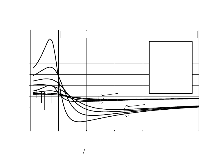
Fig. 6. Temperature drop due to JT effect
JT
T when measuring flow rate of natural
gas mixture through orifice plate with corner taps (ISO-5167, 2003). The upstream pressure
varies from 1 MPa to 60 MPa in 1 MPa steps and upstream temperature from 245 K to 305 K
in 20 K steps for each of the two differential pressures Δp (20 kPa and 100 kPa). The internal
diameters of orifice and pipe are: d=120 mm and D=200 mm.
Natural Gas518
illustrates the temperature drop caused by the JT effect and calculated in accordance with
the Eq. (44). The calculated results are given for two discrete differential pressures (
p ),
20kPa and 100kPa, for absolute pressure (p
u
) ranging from 1 MPa to 60 MPa in 1 MPa steps
and for six equidistant upstream temperatures (T
u
) in the range from 245 to 345 K. From Fig.
6 it can be seen that for each temperature there exists the corresponding pressure where JT
coefficient changes its sign and consequently alters the sign of the temperature change. A
relative error in the flow rate measurements due to JT effect is shown in Fig. 7. The error is
calculated in accordance with Eq. (46) by comparing the approximate mass flow rate (q
d
)
with the precisely calculated mass flow rate (q
u
). The approximate flow rate and the
corresponding natural gas properties (density, viscosity and isentropic exponent) are
calculated at upstream pressure p
u
, downstream temperature T
d
and differential pressure
p, by neglecting the temperature drop due to JT effect (
ud
TT ). The results are shown for
two discrete differential pressures (
p
), 20kPa and 100kPa, for absolute upstream pressure
(p
u
) ranging from 1 MPa to 60 MPa in 1 MPa steps and for four equidistant downstream
temperatures (T
d
) in the range from 245 to 305 K.
-0.05
0.00
0.05
0.10
0.15
0.20
0.25
0.30
0.35
0 10 20 30 40 50 60
Pressure p [MPa]
Relative error
E
r
=(q
m
2
-q
m
1
)/q
m
1
[%]
245K
265K
285K
305K
245K
265K
285K 305K
p=100kPa
p=20kPa
Natural gas analysis
(mole percent):
methane............85.90
ethane.................8.50
propane...............2.30
carbon dioxide.....1.50
nitrogen...............1.00
i-butane...............0.35
n-butane..............0.35
i-pentane.............0.05
n-pentane............0.05
Joule-Thomson effect
Fig. 7. Relative error
uudr
qqqE in the flow rate of natural gas measured by orifice
plate with corner taps (ISO-5167, 2003) when calculating flow rate using downstream
temperature with no compensation of JT effect (q
d
) instead of upstream temperature (q
u
).
The upstream pressure varies from 1 MPa to 60 MPa in 1 MPa steps and downstream
temperature from 245 K to 305 K in 20 K steps for each of two differential pressures Δp (20
kPa and 100 kPa). The internal diameters of orifice and pipe are: d=120 mm and D=200 mm.
Fig. 8 illustrates the relative error in the flow rate measurements due to the approximation
of the isentropic exponent by the ratio of the ideal molar heat capacities. The error is
calculated by comparing the approximate mass flow rate (q
d
) with the precisely calculated
mass flow rate (q
u
) in accordance with Eq. (46). The procedure for the precise correction of
the mass flow rate is shown in Table 5. The approximate flow rate calculation is carried out
in the same way with the exception of the isentropic exponent, which equals the ratio of the
ideal molar heat capacities (
Rcc
pImpIm
,,
). The results are shown for two discrete
differential pressures p
(20kPa and 100kPa), for absolute upstream pressure p
u
ranging
from 1 MPa to 60 MPa in 1 MPa steps and for four equidistant downstream temperatures T
d
in the range from 245 to 305 K.
-0.16
-0.14
-0.12
-0.10
-0.08
-0.06
-0.04
-0.02
0.00
0.02
0 10 20 30 40 50 60
Pressure p[MPa]
Relative error (
q
m2
-
q
m1
)/
q
m
1
[%]
245K
265K
285K
305K
245K
265K
285K
305K
p=100kPa
p=20kPa
Isentropic exponent effect
Natural gas analysis
(mole percent):
methane............85.90
ethane.................8.50
propane...............2.30
carbon dioxide.....1.50
nitrogen...............1.00
i-butane...............0.35
n-butane..............0.35
i-pentane.............0.05
n-pentane............0.05
Fig. 8. Relative error
uudr
qqqE
in the flow rate of natural gas mixture measured by
orifice plate with corner taps (ISO-5167, 2003) when using the isentropic exponent of ideal
gas (q
d
) instead of real gas (q
u
). The upstream pressure varies from 1 MPa to 60 MPa in 1
MPa steps and downstream temperature from 245 K to 305 K in 20 K steps for each of two
differential pressures Δp (20 kPa and 100 kPa). The internal diameters of orifice and pipe are:
d=120 mm and D=200 mm.
Fig. 9 shows the flow rate measurement error produced by the combined effect of the JT and
isentropic expansion. The error, Eq. (46), is calculated by comparing the approximate mass
flow rate (q
d
) with the mass flow rate (qu) calculated precisely in accordance with the
procedure depicted in Table 5. The approximate flow rate and the corresponding natural gas
properties are calculated at upstream pressure p
u
, downstream temperature T
d
and
differential pressure p, by neglecting the temperature drop due to JT effect (
ud
TT ) and
by substituting the isentropic exponent by the ratio of the ideal molar heat capacities,
Rcc
pImpIm
,,
. The results are shown for two discrete differential pressures p
(20kPa and 100kPa), for absolute upstream pressure p
u
ranging from 1 MPa to 60 MPa in 1
Natural gas properties and ow computation 519
illustrates the temperature drop caused by the JT effect and calculated in accordance with
the Eq. (44). The calculated results are given for two discrete differential pressures (
p ),
20kPa and 100kPa, for absolute pressure (p
u
) ranging from 1 MPa to 60 MPa in 1 MPa steps
and for six equidistant upstream temperatures (T
u
) in the range from 245 to 345 K. From Fig.
6 it can be seen that for each temperature there exists the corresponding pressure where JT
coefficient changes its sign and consequently alters the sign of the temperature change. A
relative error in the flow rate measurements due to JT effect is shown in Fig. 7. The error is
calculated in accordance with Eq. (46) by comparing the approximate mass flow rate (q
d
)
with the precisely calculated mass flow rate (q
u
). The approximate flow rate and the
corresponding natural gas properties (density, viscosity and isentropic exponent) are
calculated at upstream pressure p
u
, downstream temperature T
d
and differential pressure
p, by neglecting the temperature drop due to JT effect (
ud
TT
). The results are shown for
two discrete differential pressures (
p
), 20kPa and 100kPa, for absolute upstream pressure
(p
u
) ranging from 1 MPa to 60 MPa in 1 MPa steps and for four equidistant downstream
temperatures (T
d
) in the range from 245 to 305 K.
-0.05
0.00
0.05
0.10
0.15
0.20
0.25
0.30
0.35
0 10 20 30 40 50 60
Pressure p [MPa]
Relative error
E
r
=(q
m
2
-q
m
1
)/q
m
1
[%]
245K
265K
285K
305K
245K
265K
285K 305K
p=100kPa
p=20kPa
Natural gas analysis
(mole percent):
methane............85.90
ethane.................8.50
propane...............2.30
carbon dioxide.....1.50
nitrogen...............1.00
i-butane...............0.35
n-butane..............0.35
i-pentane.............0.05
n-pentane............0.05
Joule-Thomson effect
Fig. 7. Relative error
uudr
qqqE
in the flow rate of natural gas measured by orifice
plate with corner taps (ISO-5167, 2003) when calculating flow rate using downstream
temperature with no compensation of JT effect (q
d
) instead of upstream temperature (q
u
).
The upstream pressure varies from 1 MPa to 60 MPa in 1 MPa steps and downstream
temperature from 245 K to 305 K in 20 K steps for each of two differential pressures Δp (20
kPa and 100 kPa). The internal diameters of orifice and pipe are: d=120 mm and D=200 mm.
Fig. 8 illustrates the relative error in the flow rate measurements due to the approximation
of the isentropic exponent by the ratio of the ideal molar heat capacities. The error is
calculated by comparing the approximate mass flow rate (q
d
) with the precisely calculated
mass flow rate (q
u
) in accordance with Eq. (46). The procedure for the precise correction of
the mass flow rate is shown in Table 5. The approximate flow rate calculation is carried out
in the same way with the exception of the isentropic exponent, which equals the ratio of the
ideal molar heat capacities (
Rcc
pImpIm
,,
). The results are shown for two discrete
differential pressures p
(20kPa and 100kPa), for absolute upstream pressure p
u
ranging
from 1 MPa to 60 MPa in 1 MPa steps and for four equidistant downstream temperatures T
d
in the range from 245 to 305 K.
-0.16
-0.14
-0.12
-0.10
-0.08
-0.06
-0.04
-0.02
0.00
0.02
0 10 20 30 40 50 60
Pressure p[MPa]
Relative error (
q
m2
-
q
m1
)/
q
m
1
[%]
245K
265K
285K
305K
245K
265K
285K
305K
p=100kPa
p=20kPa
Isentropic exponent effect
Natural gas analysis
(mole percent):
methane............85.90
ethane.................8.50
propane...............2.30
carbon dioxide.....1.50
nitrogen...............1.00
i-butane...............0.35
n-butane..............0.35
i-pentane.............0.05
n-pentane............0.05
Fig. 8. Relative error
uudr
qqqE in the flow rate of natural gas mixture measured by
orifice plate with corner taps (ISO-5167, 2003) when using the isentropic exponent of ideal
gas (q
d
) instead of real gas (q
u
). The upstream pressure varies from 1 MPa to 60 MPa in 1
MPa steps and downstream temperature from 245 K to 305 K in 20 K steps for each of two
differential pressures Δp (20 kPa and 100 kPa). The internal diameters of orifice and pipe are:
d=120 mm and D=200 mm.
Fig. 9 shows the flow rate measurement error produced by the combined effect of the JT and
isentropic expansion. The error, Eq. (46), is calculated by comparing the approximate mass
flow rate (q
d
) with the mass flow rate (qu) calculated precisely in accordance with the
procedure depicted in Table 5. The approximate flow rate and the corresponding natural gas
properties are calculated at upstream pressure p
u
, downstream temperature T
d
and
differential pressure p, by neglecting the temperature drop due to JT effect (
ud
TT ) and
by substituting the isentropic exponent by the ratio of the ideal molar heat capacities,
Rcc
pImpIm
,,
. The results are shown for two discrete differential pressures p
(20kPa and 100kPa), for absolute upstream pressure p
u
ranging from 1 MPa to 60 MPa in 1
Natural Gas520
MPa steps and for four equidistant downstream temperatures T
d
in the range from 245 to
305 K.
-0.15
-0.10
-0.05
0.00
0.05
0.10
0.15
0.20
0.25
0.30
0 10 20 30 40 50 60
Pressure p[MPa]
Relative error (
q
m2
-
q
m1
)/
q
m
1
[%]
245K
265K
285K
305K
245K
265K
285K
305K
p=100kPa
p
=20kPa
Natural gas analysis
(mole percent):
methane............85.90
ethane.................8.50
propane...............2.30
carbon dioxide.....1.50
nitrogen...............1.00
i-butane...............0.35
n-butane..............0.35
i-pentane.............0.05
n-pentane............0.05
A combined effect of Joule-Thomson coefficient and isentropic exponent
Fig. 9. Relative error
uudr
qqqE in the flow rate of natural gas mixture measured by
orifice plate with corner taps (ISO-5167, 2003) when using downstream temperature with no
compensation of JT effect and the isentropic exponent of ideal gas at downstream
temperature (q
d
) instead of upstream temperature and the corresponding real gas isentropic
exponent (q
u
). The upstream pressure varies from 1 MPa to 60 MPa in 1 MPa steps and
downstream temperature from 245 K to 305 K in 20 K steps for each of two differential
pressures Δp (20 kPa and 100 kPa). The internal diameters of orifice and pipe are: d=120 mm
and D=200 mm.
The results obtained for JT coefficient and isentropic exponent are in a complete agreement
with the results obtained when using the procedures described in (Marić, 2005) and (Marić
et al., 2005), which use a natural gas fugacity to derive the molar heat capacities. The
calculation results are shown up to a pressure of 60 MPa, which lies within the wider ranges
of application given in (ISO-12213-2, 2006), of 0 - 65 MPa. However, the lowest uncertainty
for compressibility is for pressures up to 12 MPa and no uncertainty is quoted in reference
(ISO-12213-2, 2006) for pressures above 30 MPa. Above this pressure, it would therefore
seem sensible for the results of the JT and isentropic exponent calculations to be used with
caution. From Fig. 9 it can be seen that the maximum combined error is lower than the
maximum individual errors because the JT coefficient (Fig. 7) and the isentropic exponent
(Fig. 8) show the counter effects on the flow rate error. The error always increases by
decreasing the natural gas temperature. The total measurement error is still considerable
especially at lower temperatures and higher differential pressures and can not be
overlooked. The measurement error is also dependent on the natural gas mixture. For
certain mixtures, like natural gas with high carbon dioxide content, the relative error in the
flow rate may increase up to 0.5% at lower operating temperatures (245 K) and up to 1.0% at
very low operating temperatures (225 K). Whilst modern flow computers have provision for
applying a JT coefficient and isentropic exponent correction to measured temperatures, this
usually takes the form of a fixed value supplied by the user. Our calculations show that any
initial error in choosing this value, or subsequent operational changes in temperature,
pressure or gas composition, could lead to significant systematic metering errors.
8. Flow rate correction factor meta-modeling
Precise compensation of the flow rate measurement error is numerically intensive and time-
consuming procedure (Table 5) requesting double calculation of the flow rate and the
properties of a natural gas. In the next section it will be demonstrated how the machine
learning and the computational intelligence methods can help in reducing the complexity of
the calculation procedures in order to make them applicable to real-time calculations. The
machine learning and the computationally intelligence are widely used in modeling the
complex systems. One possible application is meta-modeling, i.e. construction of a
simplified surrogate of a complex model. For the detailed description of the procedure for
meta-modeling the compensation of JT effect in natural gas flow rate measurements refer to
(Marić & Ivek, IEEE, Marić & Ivek, 2010).
Approximation of complex multidimensional systems by self-organizing polynomials, also
known as the Group Method of Data Handling (GMDH), was introduced by A.G.
Ivakhnenko (Ivaknenkho, 1971). The GMDH models are constructed by combining the low-
order polynomials into multi layered polynomial networks where the coefficients of the
low-order polynomials (generally 2-dimensional 2
nd
-order polynomials) are obtained by
polynomial regression. GMDH polynomials may achieve reasonable approximation
accuracy at low complexity and are simple to implement in digital computers (Marić & Ivek,
2010). Also the ANNs can be efficiently used for the approximation of complex systems
(Ferrari & Stengel, 2005). The main challenges of neural network applications regarding the
architecture and the complexity are analyzed recently (Wilamowski, 2009).
The GMDH and the ANN are based on learning from examples. Therefore to derive a meta-
model from the original high-complexity model it is necessary to (Marić & Ivek, 2010):
- generate sufficient training and validation examples from the original model
- learn the surrogate model on training data and verify it on validation data
We tailored GMDH and ANN models for a flow-computer (FC) prototype based on low-
computing-power microcontroller (8-bit/16-MHz) with embedded FP subroutines for single
precision addition and multiplication having the average ET approximately equal to 50 μs
and 150 μs, respectively.
8.1 GMDH model of the flow rate correction factor
For the purpose of meta-modeling the procedure for the calculation of the correction factor
was implemented in high speed digital computer. The training data set, validation data set
and 10 test data sets, each consisting of 20000 samples of correction factor, were randomly
sampled across the entire space of application. The maximum ET of the correction factor
surrogate model in our FC prototype was limited to 35 ms (T
exe0
≤35 ms) and the maximum
root relative squared error (RRSE) was set to 4% (E
rrs0
≤4%). Fig. 10 illustrates a polynomial
graph of the best discovered GMDH surrogate model of the flow rate correction factor
obtained at layer 15 when using the compound error (CE) measure (Marić & Ivek, 2010). The
