Phadke A.G., Thorp J.S. Synchronized Phasor Measurements and Their Applications

Подождите немного. Документ загружается.

154 Chapter 7 State Estimation

ider the phasor measurements sequen-

tially with the traditional SCADA scan; that is, form the conventional es-

timate, take it and its covariance matrix and then imagine the phasor meas-

urements as in Section 7.5.1.as an addition. We can imagine combining the

two with a measurement equation of the form

[]

⎥

⎦

⎤

⎢

⎣

⎡

⎟

⎠

⎞

⎜

⎝

⎛

⎥

⎦

⎤

⎢

⎣

⎡

⎥

⎦

⎤

⎢

⎣

⎡

⎥

⎦

⎤

⎢

⎣

⎡

−

(1)

0HWH

CovE

(7.42)

where

)1(

E is the estimate from the conventional estimator and

is the re-

sidual from the linear measurements. The old covariance matrix is in polar

coordinates while the new must be converted from rectangular to polar. It

can be shown that the solution to Eq. (7.42) is the same as the solution of

[]

⎥

⎦

⎤

⎢

⎣

⎡

⎟

⎠

⎞

⎜

⎝

⎛

⎥

⎦

⎤

⎢

⎣

⎡

⎥

⎦

⎤

⎢

⎣

⎡

⎥

⎦

⎤

⎢

⎣

⎡

covE

(7.43)

which is a nonlinear hybrid estimate handling both the traditional SCADA

measurements and the phasor measurements.

7.5.3 Incomplete observability estimators

One of the disadvantages of traditional state estimators is that at the very

minimum a complete tree of the network must be monitored in order to ob-

tain a state estimate. The phasor-based estimators have the advantage that

each measurement can stand on its own, and a relatively small number of

measurements can be used directly if the application requirements could be

met. For example, consider the problem of controlling oscillations between

two systems separated by great distance. In this case, only two measure-

ments would be sufficient to provide a useful feedback signal

But in terms of a state estimator application using only PMUs the obvi-

ous question is how many PMUs need to be installed in order to measure

the state of the system using line currents as discussed in Section 7.5.1.

Given the number of lines connecting to each node in a power system is

approximately 3 it is clear that a PMU is not necessary at every bus.

The light gray buses in Figure 7.12 are unobservable to a depth of 1 in

the sense that they are only one bus away from an observable bus. It is

possible to imagine having so few PMUs that depths of unobservability of

2 or 3 or more were achieved. Algorithms to find PMU placements to

minimize the number of PMUs for a given depth have been developed [5].

The complete observability case has been approached in a number of

in Section 7.5.1 it is possible to cons

7.5 State estimation with Phasors measurements 155

Fig. 7.11 Two PMUs used to observe a nine-bus system. The larger circles repre-

sent PMUs while the smaller circles are shaded to indicate which PMU is respon-

sible for the current measurement.

ways with a consensus that PMUs are required at approximately one-third

of the buses to obtain complete observabilty. Some examples are given in

Table 7.2

Fig. 7.12 Unobservable buses.

Incidence matrices

The techniques used in [5] involve enumerating trees and can become time

consuming as system size increases. The number of possible trees for a

1500-bus system is overwhelming. The idea of searching a tree is appeal-

ing when attempting to determine PMU locations which have a certain

depth of observability. If only complete observability is of interest the

techniques in [6, 7] are more efficient. These calculations involve integer

PMU1

PMU2

PMU

Indirectly

observed

Unobserved

156 Chapter 7 State Estimation

programming and the network incidence matrix. The incidence matrix ap-

proach can also be extended to degrees of observability. Consider the net-

work graph shown in Figure 7.13. The incidence matrix is a square matrix

with

Table 7.2 Observability results for a few systems [5]

Test system Size

(Buses/Lines)

Complete

observability

Depth

IEEE 14 Bus (14,20) 3 2 2 1

IEEE 30 Bus (30,41) 7 4 3 2

IEEE 57 Bus (57,80) 11 9 8 7

System α

(270,326) 90 62 56 45

System β

(444,574) 121 97 83 68

the dimension of the number of buses. There is a one on each diagonal and

a one in the

ij the position if bus i is connected to bus j. The matrix for the

network is given by Eq. (7.44). If we imagine placing a PMU at bus 3, for

example we would learn the voltages at buses 2, 3, 4, and 6 which happens

to be the non-zero entries in column 3 of

⎥

⎦

⎤

⎢

⎣

⎡

11010000

11000010

00100101

10011000

00011100

00101110

01000111

00100011

(7.44)

7.5 State estimation with Phasors measurements 157

Fig. 7.13

A network graph.

In [6] the problem of locating the minimum number of PMUs to com-

pletely observe the network is stated as an integer programming problem

in the form

[]

min

subject to , 1 or 0

111 1

x≥=

Ax 0

(7.45)

The form in Eq. (7.45) is the simplest binary integer programming prob-

lem. Equality constraints can be added and conventional injection and flow

measurements can be accommodated [7]. The depth of observability calcu-

lation, however, was not considered in the approach. It is surprisingly easy

to include by considering the effect of taking powers of the A matrix. In

[12] it is stated that

Theorem

The ij entry in the nth power of the incidence matrix for any

graph or diagraph is exactly the number of different paths of length n, be-

ginning at vertex i and ending at vertex j.

The proof is by induction and is easy to see in our example. The signum of

is the incidence matrix of another graph which has branches added to

the graph in Figure 7.13 as shown in Figure 7.14. The network associated

with A

for this example has all nodes connected to all other nodes. In a

“small world” context the example has four degrees of separation, that is,

1 2 3 4 5

7 8

1 2 3 4 5

7 8

158 Chapter 7 State Estimation

every node can be reached from any other node by going through four

branches.

⎥

⎦

⎤

⎢

⎣

⎡

32021010

23010121

00301222

21032100

10123210

01212422

12201242

01100223

(7.46)

The 1–5 path is such an example. In terms of depth of unobservability, a

single PMU at nodes 2, or 3, or 4, or 7 gives a depth of unobservability of

3. The number of paths is not important in placing PMUs so the sgn(A

)

plays the role of A in the integer programming formulation for the depth of

observability problem.

Fig. 7.14 The graph of sgn (A*A).

A common problem is to determine the optimum phased deployment of

PMUs. There is usually a limited annual budget to put a certain number of

PMUs in place each year. The ultimate goal is to have a completely ob-

servable system of measurements at the end of a multiyear time window.

It would be best if the PMUs installed in the first year represented a good

choice given the small number involved. For example, a set of PMUs that

gave some degree of unobservability in each year with a progression to

1 2 3 4 5

7 8

1 2 3 4 5

7 8

1 2 3 4 5

7 8

7.5 State estimation with Phasors measurements 159

complete observability at the end of period would be ideal. The incidence

matrix approach offers a convenient solution to this problem. Suppose x

is a solution of the complete observability calculation in Eq. (7.45) and

consider

[]

1111

,)][sgn(tosubject

min

=−

≥

x)x(f

0xAA

(7.47)

The use of sgn(AA) assures the solution has depth of observability of 1

and the equality constraint says x

must be chosen from the locations in x

For a large system a great deal of computation is involved in solving for x

while x

is much quicker and succeeding solutions are quicker yet. The

general form is in Eq. (7.48):

0)][sgn(tosubject

min

=−

≥

−

x)x(f

(7.48)

For the 57-bus system studied in [5] and [6] there are 15 “zero injection

buses” (buses with no generation or load). The different treatments of

these buses produce slight variation in the results. The technique in [5]

produced the numbers in Table 7.2. If the zero injection buses are simple

reduced by network equivalencing a 42-bus network is created. The 42-

bus network is more “connected” than the original because the elimination

of a bus that has connections to both buses

p and q produces a new line

from

p to q. The elimination of 15 buses creates a number of additional

lines. The repeated application of Eq. (7.48) produces a nested solution for

the reduced network but if the reduced network is too different from the

original network there are still unanswered questions for the original net-

work.

A reasonable approach is to limit the network reductions to obvious sit-

uations. An example system has 1443 buses and 1929 branches. There are

104 buses that have three or fewer branches connected to them. If they are

eliminated by network reduction the number of branches grows to 2178

and the nested solution is shown in Table 7.3. If only the five buses with

only two branches are removed the number of branches grows to 1940 and

the computation takes considerably longer. Again the results are in Table

7.3.

160 Chapter 7 State Estimation

Table 7.3 Observability results two versions of the 1246-bus system

# Con-

nections

to buses

removed

(Buses

/Lines)

Depth

1 or 2 or3 (1339/2178) 433 218 131 74 54 43

1 or 2 (1458/1940) 445 248 135 83 61 42

7.5.4 Partitioned state estimation

Some have suggested that the only optimum answer to these problems

is to start over and pool the models and data and buy more computers. If

a simpler solution which saves money, time, and frustration can be found

it certainly seems worth considering. Consider the system in Figure 7.15.

The boundary buses in Figure 7.15 could be the high sides of transform-

ers connecting high- and low-voltage subsystems or the buses at the end

of the tie lines between ISOs. An attractive approach to the problem is to

let each system use their existing state estimator but recognize that the

two estimators do have different references. By including the boundary

buses in both systems we can estimate the difference between the two

references. If NB is the number of boundary buses, and sub 1 and 2 de-

note estimates from each side then

is the estimated difference between

the two references.

Early state estimators were restricted to the highest voltage levels and did

not extend to voltages as high as 138 kV in some utilities. The advent of

PMU technology made it possible to imagine using the existing conven-

tional estimator supplemented by PMU measurements in portions of the

lower voltage system. Again because a few PMU measurements are useful

it is not necessary to fully measure the low-voltage network. A second

more recent problem of the same type is the seams issue. Two adjoining

ISOs with large and elaborate state estimation programs representing im-

mense investment in people and systems would like to combine their state

estimates. Typically the people who would actually have to do it have the

most reservations. Given the size of an independent system operator (ISO)

estimator some reservations are justified. Combining two 30 000 bus esti-

mators which probably work differently and their own quirks is a daunting

prospect. Both problems involve the concept of joining state estimators.

7.5 State estimation with Phasors measurements 161

Fig. 7.15 Two systems with boundary buses.

12,

ˆˆ

()

θθ

=−

∑

(7.49)

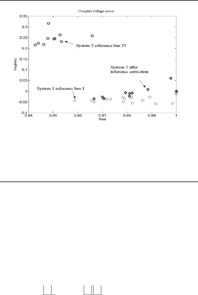
Example 7.5

The 30 bus system is divided into two subsystems as shown in Figure 7.16.

Two estimators are formed using the tie-line flows as sources or

.Fig. 7.16 The 30-bus system divided into two subsystems.

System 2

System 1

Boundary

Buses

162 Chapter 7 State Estimation

Fig. 7.17 The voltage errors before and after correction.

loads. The reference for system 1 is bus 1 as before but the reference for

system 2 is bus 23. The voltage errors are shown in Figure 7.17. The dia-

monds show the corrected errors in system 2 after the reference is esti-

mated.

7.5.4.1 Nonlinear residual minimization method

aab

ab ab

cos( ) cos( )

Cz z

VVV

θδ φ

=− +−

(7.50)

A study of alternative approaches to integrating adjoining estimators is in

[13] where the solution that combines small computational burden, accu-

racy, and robustness was chosen as the “nonlinear residual minimization”

(NLRM). Let the subscript C denote calculated quantities given and N be

the total number of tie lines between the two systems. The calculated quan-

tities for a line from node a to node b are given by Eqs. (7.50) and (7.51).

In the method (NLRM) the angle difference between systems,

, was cho-

sen to minimize J(

)in Eq. (7.52). In Eq. (7.52) the subscript m denotes

measured quantities.

7.5 State estimation with Phasors measurements 163

aaabab

sin( ) sin( )

Cz z

VVBVV

θδ φ

=+− +−

(7.51)

)(

CNmN

φJ

−

(7.52)

Using Eq. (7.52) with

abz

θδ

φηφηφη

sincoscossin)sin(

sinsincoscos)cos(

−=−

−

(7.53)

Then the objective function is given by Eq. (7.54):

sincos)(

φφφ

ZYXJ ++=

(7.54)

Since X, Y, and Z are constants Eq. (7.54) is equivalent to Eq. (7.55) where

A, B, C, D, and E are constants:

φφφφφφφ

sincossincossincos)( EDCBAJ ++++=

(7.55)

The minimization of Eq. (7.55) involves taking the first derivative with

respect to

, equating it to zero and using Newton’s method to solve the

resulting scalar nonlinear equation.