Pao Y.C. Engineering Analysis: Interactive Methods and Programs with FORTRAN, QuickBASIC, MATLAB, and Mathematica

Подождите немного. Документ загружается.

Engineering

Analysis

Interactive Methods and Programs

with FORTRAN, QuickBASIC, MATLAB,

and Mathematica

Y. C. Pao

Boca Raton London New York Washington, D.C.

CRC Press

Acquiring Editor:

Cindy Renee Carelli

Project Editor:

Albert W. Starkweather, Jr.

Cover design:

Dawn Boyd

Library of Congress Cataloging-in-Publication Data

Catalog record is available from the Library of Congress

This book contains information obtained from authentic and highly regarded sources. Reprinted

material is quoted with permission, and sources are indicated. A wide variety of references are listed.

Reasonable efforts have been made to publish reliable data and information, but the author and the

publisher cannot assume responsibility for the validity of all materials or for the consequences of their use.

Neither this book nor any part may be reproduced or transmitted in any form or by any means,

electronic or mechanical, including photocopying, microﬁlming, and recording, or by any information

storage or retrieval system, without prior permission in writing from the publisher.

The consent of CRC Press LLC does not extend to copying for general distribution, for promotion,

for creating new works, or for resale. Speciﬁc permission must be obtained in writing from CRC Press

LLC for such copying.

Direct all inquiries to CRC Press LLC, 2000 Corporate Blvd., N.W., Boca Raton, Florida 33431.

Trademark Notice:

Product or corporate names may be trademarks or registered trademarks, and are

only used for identiﬁcation and explanation, without intent to infringe.

Mathematica

is developed by Wolfram Research, Inc., Champaign, IL.

Windows

is developed by Microsoft Corp., Redmond, WA.

No claim to original U.S. Government works

International Standard Book Number 0-8493-2016-X

Printed in the United States of America 1 2 3 4 5 6 7 8 9 0

Printed on acid-free paper

Files Available from CRC Press

FORTRAN

QuickBASIC

MATLAB

, and Mathematic ﬁles, which contain the

source and executable programs associated with this book are available from CRC

Press’ website — http://www.crcpress.com.

Before downloading, prepare two 3.5-inch, high-density disks — one for the

ﬁles and one for a backup. Also create a temporary directory named <interactive>

on your hard drive, which will expedite downloading. To download these ﬁles, type:

http://www.crcpress.com/us/ElectronicProducts/downandup.asp.

When prompted, enter

2016

under name and

crcpress

under password. Then store the ﬁles in the

<interactive> folder. If you encounter a problem, call 1-800-CRC-PRES (272-7737).

The dowloaded ﬁles may be copied to a 3.5-inch disk. The temporary <interactive>

folder then may be deleted. Don’t forget to make a backup copy of your 3.5-inch disk.

There are four subdirectories

<QB>

, and

<Math-

tica>

which contain the

FORTRAN

source and executable programs,

QuickBASIC

source and executable programs,

ﬁles of

MATLAB

, and input and output state-

ments of for the

Mathematica

operations depicted in this textbook, respectively:

has the following ﬁles:

EDITFOR.EXE is provided for re-editing the *.FOR source programs such as

Bairstow.FOR, CubeSpln.FOR, etc. (refer to the

FORTRAN

programs index) to

include supplementary subprograms describing the problem which need to be solved

interactively. To re-edit, insert the 3.5-inch disk into Drive A and when the a:\ prompt

shows, type cd fortran to switch to the

subdirectory. For example,

to solve a polynomial by the Bairstow’s method one needs to deﬁne the polynomial,

for which the roots are to be computed. To reedit Bairstow.FOR, the user enters

a:\editfor Bairstow.for to add new

FORTRAN

statements or change them. Notice

that both upper and lower case characters are acceptable. While creating a new

version of Bairstow.FOR, the old version will be saved in Bairstow.BAK.

To create an object ﬁle, FOR1 ﬁlename such as Bairstow.FOR and FOR2 need

to be implemented. A BAISTOW.OBJ will then be generated. For linking with the

FORTRAN

library functions,

FORTRAN

.LIB, one enters, for example, LINK

Bairstow to create an executable ﬁle Bairstow.EXE. To

run

, the user simply types

Bairstow after the prompt A:\ and then answers questions interactively.

Bairstow.FOR CharacEquationFOR CubeSpln.FOR DiffTabl.FOR

EditFOR.EXE EigenVec.FOR EigenvIt.FOR ExactFit.FOR

FindRoot.FOR FOR1.EXE FOR2.EXE FORTRAN.LIB

Gauss.FOR GauJor.FOR LagrangI.FOR LeastSq1.FOR

LeastSqG.FOR LINK.EXE MatxInvD.FOR NewRaphG.FOR

NuIntgra.FOR OdeBvpFD.FOR OdeBvpRK.FOR ParabPDE.FOR

Relaxatn.FOR RungeKut.FOR Volume.FOR WavePDE.FOR

has the following ﬁles:

To commence

QuickBASIC

, when a:\ is prompted on screen, the user enters

QB. QB.EXE and BRUN40.EXE therefore are included in

<QB>

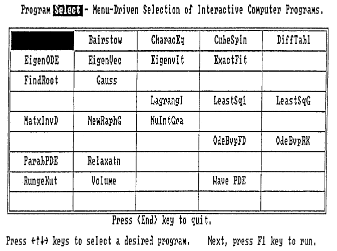
. The program

Select

enables user to select the available

QuickBASIC

program in this textbook.

After user responds with C:\Select, the screen shows a menu as shown in Figure 1

and user then follow the screen help-messages to run a desired program.

is a subdirectory associated with

MATLAB

and has the following

ﬁles:

When the 3.5-inch disk containing all of these

ﬁles is in Drive A, any of these

ﬁles can be accessed by enclosing the ﬁlename inside a pair of parentheses as

illustrated in

Section 3.2

where F.m and FP.m are required for FindRoot.m and in

Section 5.2

where an integrand function

integrnd.m

is deﬁned for numerical inte-

gration. If all ﬁles have been added into

MATLAB

library m ﬁles, then no reference

to the Drive A is necessary and the pair of parentheses can also be dropped.

is a subdirectory associated with

Mathematica

and has the ﬁles of:

Select.BAS Select.EXE

Bairstow.EXE BRUN40.EXE CharacEq.EXE CubeSpln.EXE

EigenStb.EXE EigenVec.EXE EigenVib.EXE EigenvIt.EXE

ExactFit.EXE FindRoot.EXE Gauss.EXE LagrangI.EXE

LeastSq1.EXE LeastSqG.EXE MatxInvD.EXE NuIntgra.EXE

OdeBvpFD.EXE OdeBvpRK.EXE ParabPDE.EXE QB.EXE

Relaxatn.EXE RungeKut.EXE Volume.EXE

Bairstow.QB CharacEq.QB CubeSpln.QB DiffTabl.QB

EigenStb.QB EigenVec.QB EigenVib.QB EigenvIt.QB

ExactFit.QB FindRoot.QB GauJor.QB Gauss.QB

LagrangI.QB LeastSq1.QB LeastSqG.QB MatxAlgb.QB

MatxMtpy.QB NewRaphG.QB NuIntgra.QB OdeBvpFD.QB

OdeBvpRK.QB ParabPDE.QB Relaxatn.QB RungeKut.QB

Volume.QB WavePDE.QB

BVPF.m DerivatF.m DiffTabl.m EigenvIt.m

F.m FindRoot.m FP.m Functns.m

FuncZ.m FuncZnew.m FunF.m GauJor.m

integrnd.m LagrangI.m LeastSqG.m NewRaphG.m

ParabPDE.m Relaxatn.m Volume.m Warping.m

WavePDE.m

Bairstow.MTK CubeSpln.MTK DiffTabl.MTK EigenVec.MTK

ExactFit.MTK FindRoot.MTK FUNCTNS.MTK EigenvIt.MTK

Gauss.MTK GauJor.MTK LagrangI.MTK LeastSq1.MTK

LeastSqG.MTK MatxAlgb.MTK NewRaphG.MTK NuIntgra.MTK

OdeBvpFD.MTK OdeBvpRK.MTK ParabPDE.MTK Rexalatn.MTK

RungeKut.MTK Volume.MTK WavePDE.MTK

Any of the above programs can be executed by

Mathematica

via mouse oper-

ation. First, by clicking the

File

option and when the pull-down menu appears, select

Open

and then enter the ﬁlename such as a:\Mathtica\MatxAlgb.MTK (assuming

the 3.5-inch disk containing

is in Drive A) and press the

Enter

key.

When all lines of this ﬁle is displayed on screen, move cursor to any input line such

In[1]

: A = {{1,2},{3,4}}; MatrixForm[A] and hit the

Enter

key.

Mathematica

will respond by repeating those lines for

Out[1]

. Hence, user can reproduce all of

the output lines by sequentially running the input lines [1] through [9]. However, if

user ﬁrst run In[1] and then In[3],

Mathematica

cannot perform the addition of [A]

because [B] is not deﬁned. If after having run In[1], user selects In[5], or, In[6],

Mathematica

then has no problem of giving out results.

FIGURE 1.

The Select screen.

Dedication

This book is dedicated to Prof. E. J. Marmo,

who offered a congenial work-environment for the author

to grow in the computer-aided engineering ﬁeld.

Preface and Acknowledgments

Writing textbooks on topics in the ﬁeld of

Computer Aided Engineering

(CAE)

indeed has been a very satisfying experience. First, I had the pleasure of being a

coauthor with Prof. Thomas C. Smith of the book

Introduction to Digital Computer

Plotting

by Gordon & Breach in 1973. The book

Elements of Computer-Aided

Design and Manufacturing, CAD/CAM

, was published in 1982 by John Wiley &

Sons. The book

A First Course in Finite Element Analysis

published by Allyn &

Bacon followed in 1986, and

Engineering Drafting and Solid Modeling with Silver-

Screen,

published by CRC Press, appeared in 1993.

Having taught the subjects of computer methods for engineering analysis since

1966, I ﬁnally have the courage to organize this textbook out of a large volume of

classroom notes collected over the past 31 years.

The rapid growth of computer technology is difﬁcult for any one to keep pace,

and to make revision of textbooks in the CAE ﬁeld. However, the computational

methods developed by the pioneers, such as Euler, Gauss, Lagrange, Newton, and

Runge, continue to serve us incredibly effective. These computational algorithms

remain classic, only are now executed with modern computer technology.

As far as the programming languages are concerned,

FORTRAN

has been

dominating the scientiﬁc ﬁelds for many decades.

BASIC

considered by many to

be too plain and cumbersome while

is considered by others to be too sophisticated;

both, however, are gaining popularity and increasingly replacing

FORTRAN

in the

computational community. This is particularly true when

QuickBASIC

was intro-

duced by Microsoft.

MATLAB

and

Mathematica

developed by the MathWorks, Inc. and Wolfram

Research, Inc., respectively both contain a vast collection of ﬁles (similar to

FOR-

TRAN

’s library functions) which can perform the often-encountered computational

problems. For implementation, the

MATLAB

and

Mathematica

instructions to be

interactively entered through keyboard are extremely simple. And, it also provides

very easy-to-use graphic output. When students ﬁnd it too easy to use, they often

become uninterested in learning what are the methods involved. This text is prepared

with

FORTRAN

QuickBASIC

MATLAB

and

Mathematica

, and more impor-

tantly gives the algorithms involved in the methods. Ample number of sample

problems are solved to demonstrate how the developed programs should be inter-

actively applied. Furthermore, the development of the user-generated supplementary

ﬁles is emphasized so that more supporting subprograms can be added to the

MATLAB

m-ﬁles and

Mathematica

toolkits. It is a text for self-study as well as

for the need of general references.

Numerous friends, colleagues, and students have assisted in collecting the materials

assembled herein, and they have made a great number of constructive suggestions for

the betterment of this work. To them, I am most grateful. Especially, I would like to

thank my long-time friends Dr. H. C. Wang, formerly with the IBM Thomas Watson

Research Laboratory and now with the Industrial Research Institutes in Hsingchu,

Taiwan; Dr. Erik L. Ritman of the Mayo Clinic in Rochester, MN, and Leon Hill

of the Boeing Company in Seattle, WA, for their help and encouragement throughout

my career in the CAE ﬁeld. Profs. R. T. DeLorm, L. Kersten, C. W. Martin, R. N.

McDougal, G. M. Smith, and E. J. Marmo had assisted in acquiring equipment and

research funds which made my development in the CAE ﬁeld possible, I extend my

most sincere gratitude to these colleagues at the University of Nebraska–Lincoln.

For providing constructive inputs to my published works, I should give credits to

Prof. Gary L. Kinzel of the Ohio State University, Prof. Donald R. Riley of the

University of Minnesota, Dr. L. C. Chang of the General Motors’ EDS Division, Dr.

M. Maheshiwari and Mr. Steve Zitek of the Brunswick Corp., my former graduate

assistants J. Nikkola, T. A. Huang, K. A. Peterson, Dr. W. T. Kao, Dr. David S. S.

Shy, C. M. Lin, R. M. Sedlacek, L. Shi, J. D. Wilson, Dr. A. J. Wang, Dave Breiner,

Q. W. Dong, and Michael Newman, and former students Jeff D. Geiger, Tim Car-

rizales, Krishna Pendyala, S. Ravikoti, and Mark Smith. I should also express my

appreciation to the readers of my other four textbooks mentioned above who have

frequently contacted me and provided input regarding various topics that they would

like to be considered as connected to the ﬁeld of CAE and numerical problems that

they would like to be solved by application of computer. Such input has proven to

be invaluable to me in preparation of this text. CRC Press has been a delightful

partner in publishing my previous book and again this book. The completion of this

book would not be possible without the diligent effort and superb coordination of

Cindy Renee Carelli, Suzanne Lassandro, and Albert Starkweather, I wish to express

my deepest appreciation to them and to the other CRC editorial members. Last but

not least, I thank my wife, Rosaline, for her patience and encouragement.

Y. C. Pao

Contents

1 Matrix Algebra and Solution of Matrix Equations

1.1 Introduction

1.2 Manipulation of Matrices

1.3 Solution of Matrix Equation

1.4 Program Gauss — Gaussian Elimination Method

1.5 Matrix Inversion, Determinant, and Program MatxInvD

1.6 Problems

1.7 Reference

2 Exact, Least-Squares, and Spline Curve-Fits

2.1 Introduction

2.2 Exact Curve Fit

2.3 Program LeastSq1 — Linear Least-Squares Curve-Fit

2.4 Program LeastSqG — Generalized Least-Squares Curve-Fit

2.5 Program CubeSpln — Curve Fitting with Cubic Spline

2.6 Problems

2.7 Reference

3 Roots of Polynomial and Transcendental Equations

3.1 Introduction

3.2 Iterative Methods and Program Roots

3.3 Program NewRaphG — Generalized Newton-Raphson

Iterative Method

3.4 Program Bairstow — Bairstow Method for Finding

Polynomial Roots

3.5 Problems

3.6 References

4 Finite Differences, Interpolation, and Numerical Differentiation

4.1 Introduction

4.2 Finite Differences and Program DiffTabl — Constructing

Difference Table

4.3 Program LagrangI — Applications of Lagrangian

Interpolation Formula

4.4 Problems

4.5. Reference

5 Numerical Integration and Program Volume

5.1 Introduction

5.2 Program NuIntGra — Numerical Integration by Application of the

Trapezoidal and Simpson Rules

5.3 Program Volume — Numerical Solution of Double Integral

5.4 Problems

5.5 References

6 Ordinary Differential Equations — Initial and Boundary

Value Problems

6.1 Introduction

6.2 Program RungeKut — Application of Runge-Kutta Method

for Solving InitialValue Problems

6.3 Program OdeBvpRK — Application of Runge-Kutta Method

for Solving Boundary Value Problems

6.4 Program OdeBvpFD — Application of Finite-Difference Method

for Solving Boundary-Value Problems

6.5 Problems

6.6 References

7 Eigenvalue and Eigenvector Problems

7.1 Introduction

7.2 Programs EigenODE.Stb and EigenODE.Vib — for Solving

Stability and Vibration Problems

7.3 Program CharacEq — Derivation of Characteristic Equation

of a Speciﬁed Square Matrix

7.4 Program EigenVec — Solving Eigenvector by Gaussian

Elimination Method

7.5 Program EigenvIt — Iterative Solution of Eigenvalue

and Eigenvector

7.6 Problems

7.7 References

8 Partial Differential Equations

8.1 Introduction

8.2 Program ParabPDE — Numerical Solution of Parabolic Partial

Differential Equations

8.3 Program Relaxatn — Solving Elliptical Partial Differential

Equations by Relaxation Method

8.4 Program WavePDE — Numerical Solution of Wave Problems

Governed by Hyperbolic Partial Differential Equations

8.5 Problems

8.6 References