Ockendon J., Howison S., Lacey A., Movchan A. Applied Partial Differential Equations

Подождите немного. Документ загружается.

238 ELLIPTIC EQUATIONS

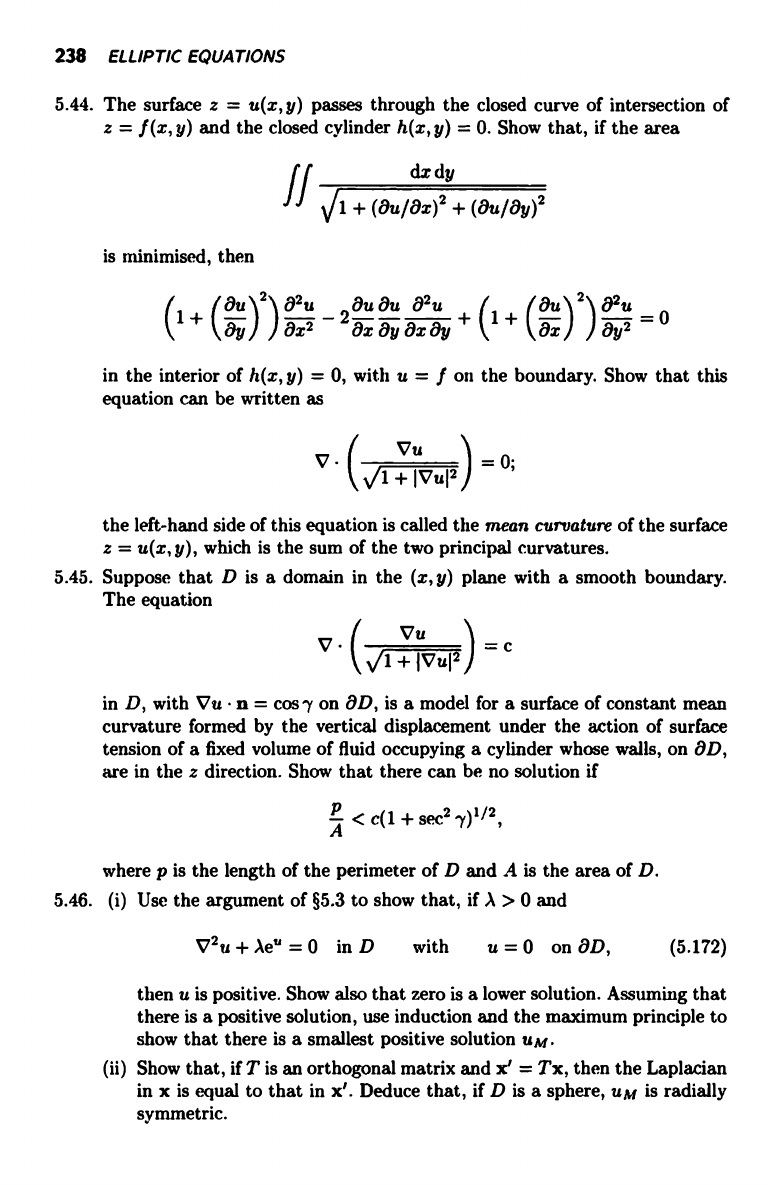
5.44. The surface z = u(x, y) passes through the closed curve of intersection of

z = f (x, y) and the closed cylinder h(x, y) = 0. Show that, if the area

dx dy

(au/ax)2 + (8u/ay)2

is minimised, then

rau

)2).92U

8uau a2u

a2u

8x2 - 2 ax ay ax ay

+ (1 +

(OU)

ax)

aye =

in the interior of h(x, y) = 0, with u = f on the boundary. Show that this

equation can be written as

l+IVuI2

the left-hand side of this equation is called the mean curvature of the surface

z = u(x, y), which is the sum of the two principal curvatures.

5.45. Suppose that D is a domain in the (x, y) plane with a smooth boundary.

The equation

TU-17)

in D, with Vu n = cosy on 8D, is a model for a surface of constant mean

curvature formed by the vertical displacement under the action of surface

tension of a fixed volume of fluid occupying a cylinder whose walls, on OD,

are in the z direction. Show that there can be no solution if

< c(1 + sect

7)1"2,

where p is the length of the perimeter of D and A is the area of D.

5.46. (i) Use the argument of §5.3 to show that, if a > 0 and

V2u + Ae' = 0

in D

with u = 0

on OD,

(5.172)

then u is positive. Show also that zero is a lower solution. Assuming that

there is a positive solution, use induction and the maximum principle to

show that there is a smallest positive solution um.

(ii) Show that, if T is an orthogonal matrix and x' = Tx, then the Laplacian

in x is equal to that in x'. Deduce that, if D is a sphere, um is radially

symmetric.

EXERCISES 239

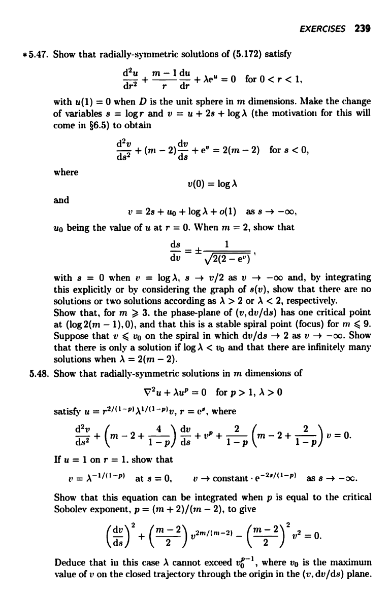
* 5.47. Show that radially-symmetric solutions of (5.172) satisfy

d2u m - ldu

dr2+ r

dr+Ae"=0 for0<r<1,

with u(1) = 0 when D is the unit sphere in m dimensions. Make the change

of variables s = log r and v = u + 2s + log A (the motivation for this will

come in §6.5) to obtain

d2u

ds2+(m-2)ds+e"=2(m-2) fors<0,

where

and

v(0) = log A

v=2s+uo+logA+o(1) ass -- -oo,

uo being the value of u at r = 0. When in = 2, show that

2(2 - et')%

with s = 0 when v = log A, s -4 v/2 as v -> -oo and, by integrating

this explicitly or by considering the graph of s(v), show that there are no

solutions or two solutions according as A > 2 or A < 2, respectively.

Show that, for m >, 3. the phase-plane of (v, dv/ds) has one critical point

at (log 2(m - 1),0), and that this is a stable spiral point (focus) for m < 9.

Suppose that v < vo on the spiral in which dv/ds - 2 as v -+ -00. Show

that there is only a solution if log A < vo and that there are infinitely many

solutions when A = 2(tn - 2).

5.48. Show that radially-symmetric solutions in m dimensions of

V2u+Aup=O fore>1,A>0

satisfy u =

r2/(1-p)A1/(1-p)v,

r = e", where

z-+ m-2+

dv+vp+

m-2+

v=0.

ds2

(

1-p ds

1-p

JIu= lonr= 1. show that

t+ =

A-1/('-p)

at s = 0,

v -+ constant - e-20/(l

-p)

ass -+ -oc.

Show that this equation can be integrated when p is equal to the critical

Sobolev exponent, p = (m + 2)/(tn - 2), to give

Cd4/

(m_2)

U2m/(m-2) -

(in_2)21,2

= 0.

Deduce that in this case A cannot exceed vo-1, where vo is the maximum

value of v on the closed trajectory through the origin in the (v, dv/ds) plane.

240 ELLIPTIC EQUATIONS

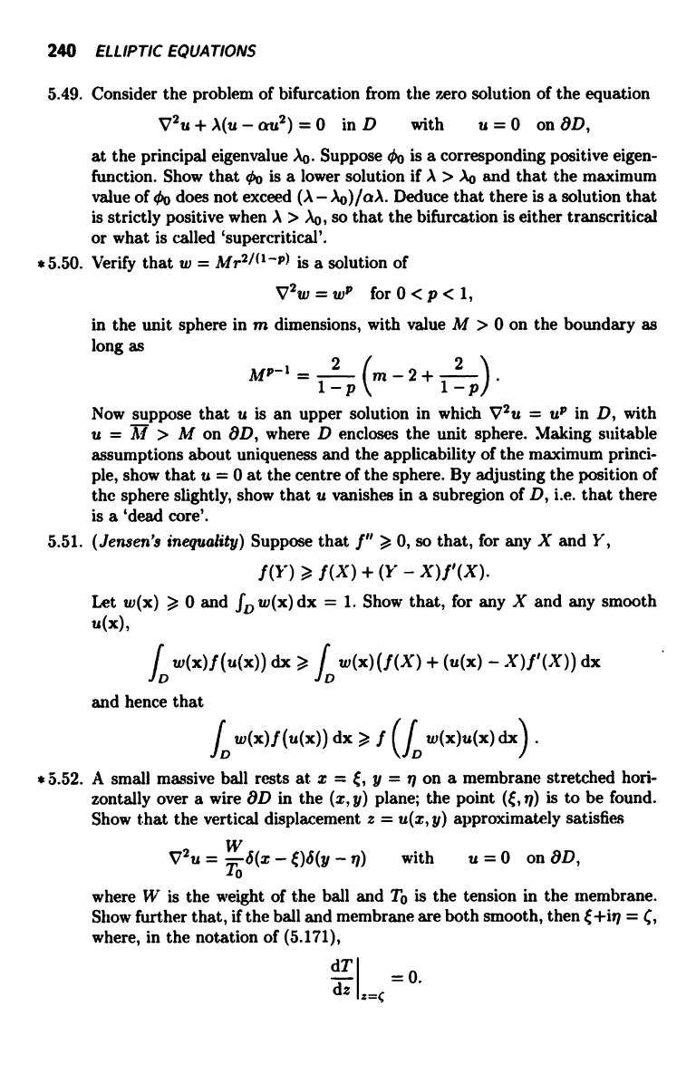
5.49. Consider the problem of bifurcation from the zero solution of the equation

V2u + A(u - cau2) = 0 in D

with

u = 0 on OD,

at the principal eigenvalue )b. Suppose 00 is a corresponding positive eigen-

function. Show that 00 is a lower solution if A > A0 and that the maximum

value of 00 does not exceed (A - Jb)/aA. Deduce that there is a solution that

is strictly positive when A > A0, so that the bifurcation is either transcritical

or what is called `supercritical'.

* 5.50. Verify that w = Mr2/('

) is a solution of

V2w=w' for0<p<1,

in the unit sphere in m dimensions, with value M > 0 on the boundary as

long as

MP-1=12p(m-2+12p).

Now suppose that it is an upper solution in which V2u = u' in D, with

u = TY > M on OD, where D encloses the unit sphere. Making suitable

assumptions about uniqueness and the applicability of the maximum princi-

ple, show that u = 0 at the centre of the sphere. By adjusting the position of

the sphere slightly, show that it vanishes in a subregion of D, i.e. that there

is a `dead core'.

5.51. (Jensen's inequality) Suppose that f" > 0, so that, for any X and Y,

f(Y)1> f(X) + (Y - X) f'(X).

Let w(x) > 0 and fD w(x) dx = 1. Show that, for any X and any smooth

u(x),

w(x) f (u(x)) dx %

w(x) (f (X) + (u(x) - X) f'(X )) dx

and hence that

f w(x) f (u(x)) dx > f I fw(x)u(x) dx) .

D \ D

* 5.52. A small massive ball rests at x = , y = n on a membrane stretched hori-

zontally over a wire 8D in the (x, y) plane; the point ({, rI) is to be found.

Show that the vertical displacement z = u(x, y) approximately satisfies

V2u =

b(x - t)b(y - 71)

with u = 0 on 8D,

To-

where W is the weight of the ball and To is the tension in the membrane.

Show further that, if the ball and membrane are both smooth, then t+iq = t;,

where, in the notation of (5.171),

- 0

z=c

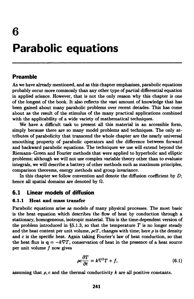
Parabolic equations

Preamble

As we have already mentioned, and as this chapter emphasises, parabolic equations

probably occur more commonly than any other type of partial differential equation

in applied science. However, that is not the only reason why this chapter is one

of the longest of the book. It also reflects the vast amount of knowledge that has

been gained about many parabolic problems over recent decades. This has come

about as the result of the stimulus of the many practical applications combined

with the applicability of a wide variety of mathematical techniques.

We have a difficult task to present all this material in an accessible form,

simply because there are so many model problems and techniques. The only at-

tributes of parabolicity that transcend the whole chapter are the nearly universal

smoothing property of parabolic operators and the difference between forward

and backward parabolic equations. The techniques we use will extend beyond the

Riemann-Green and Fourier methods that were applied to hyperbolic and elliptic

problems; although we will not use complex variable theory other than to evaluate

integrals, we will describe a battery of other methods such as maximum principles,

comparison theorems, energy methods and group invariance.

In this chapter we follow convention and denote the diffusion coefficient by D;

hence all spatial domains are denoted by Il.

6.1 Linear models of diffusion

6.1.1 Heat and mass transfer

Parabolic equations arise as models of many physical processes. The most basic

is the heat equation which describes the flow of heat by conduction through a

stationary, homogeneous, isotropic material. This is the time-dependent version of

the problem introduced in §5.1.3, so that the temperature T is no longer steady

and the heat content per unit volume, pcT, changes with time; here p is the density

and c is the specific heat. Again taking Fourier's law of heat conduction, so that

the heat flux is q = -kVT, conservation of heat in the presence of a heat source

per unit volume f now gives

pcas= kV2T + f,

assuming that p, c and the thermal conductivity k are all positive constants.

241

242

PARABOLIC EQUATIONS

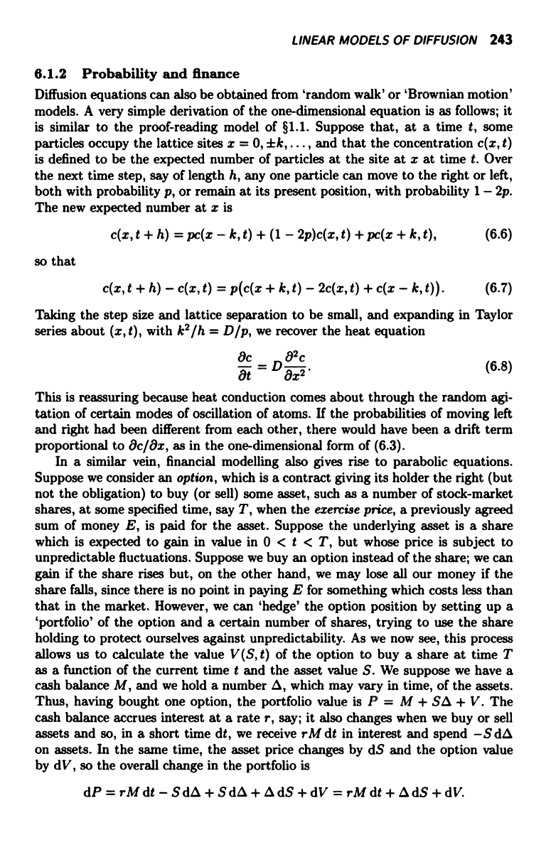
In the absence of any heat source, (6.1) reduces to

= DVZT,

(6.2)

where D = k/pc is known as the thermal diffusivity, and we will refer to both (6.1)

and (6.2) as heat equations. In both (6.1) and (6.2) we would expect to know the

distribution of T at t = 0 in addition to boundary conditions imposed on spatial

boundaries (possibly moving with finite speed) of the type described in §5.1.3.

These equations are often also referred to as diffusion equations because they

also model diffusive mass transfer. Suppose one material, say strawberry sauce, is

free to move under the sole action of molecular diffusion through another, station-

ary, material, say yoghurt, and suppose the concentration c(x, t), defined to be

the ratio of the masses of sauce and yoghurt per unit total volume, is low. Then

Fick's law relates the mass flux of the mobile phase to c by q = -DVc, where D

is called the diffusivity. Conservation of mass implies that

for constant diffusivity. If, however, the medium is moving with velocity v there

is also mass transfer by convection. We can model this either by generalising

the argument leading to (6.1) or by simply realising that the total mass flux is

q = cv - DVc, so that c satisfies the convection-diffusion equation

ac = DVzc - V. (cv),

which, if V v = 0, can be written as

(I+V.v

c=DV2C.

(6.3)

A version of (6.3) arises when modelling the distribution c of a pollutant in

a river along the x axis. With a unidirectional flow v = (v(y, z), 0, 0), we would

write

0c 0C =

z z z

+ v8x

D (8xz

+ W2 + az2 ) '

(6.4)

but it now probably makes physical sense to interpret D as representing the effects

of turbulence rather than molecular diffusion. The term 82c/8xz in (6.4) is often

ignored when the river is long, and in such cases the boundary conditions at the

downstream end of the river are ignored. When this approximation is made and

when we restrict ourselves to steady states, c satisfies

19C =

v8x D (8yz

+ 8zz I , (6.5)

which shows that time does not have to be the independent variable on the left-

hand side of a diffusion equation; in steady convection, `distance downstream' is

synonymous with `time' in conventional heat conduction.

LINEAR MODELS OF DIFFUSION 243

6.1.2

Probability and finance

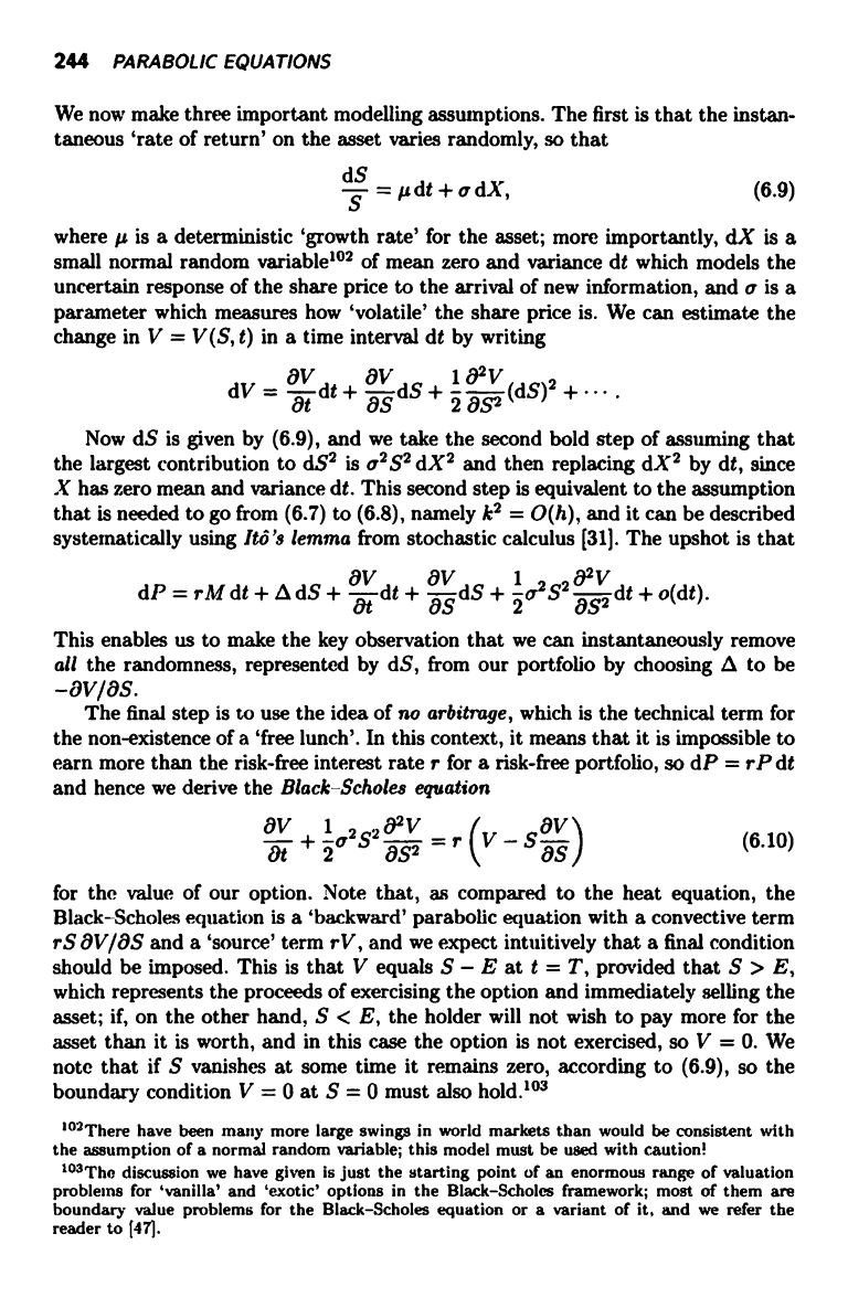
Diffusion equations can also be obtained from `random walk' or `Brownian motion'

models. A very simple derivation of the one-dimensional equation is as follows; it

is similar to the proof-reading model of §1.1. Suppose that, at a time t, some

particles occupy the lattice sites x = 0, ±k,..., and that the concentration c(x, t)

is defined to be the expected number of particles at the site at x at time t. Over

the next time step, say of length h, any one particle can move to the right or left,

both with probability p, or remain at its present position, with probability 1 - 2p.

The new expected number at x is

c(x, t + h) = pc(x - k, t) + (1 - 2p)c(x, t) + pc(x + k, t), (6.6)

so that

c(x,t + h) - c(x,t) = p(c(x + k,t) - 2c(x,t) + c(x - k,t)).

(6.7)

Taking the step size and lattice separation to be small, and expanding in Taylor

series about (x, t), with kz/h = D/p, we recover the heat equation

at =

D02C

x. (6.8)

This is reassuring because heat conduction comes about through the random agi-

tation of certain modes of oscillation of atoms. If the probabilities of moving left

and right had been different from each other, there would have been a drift term

proportional to Oc/Ox, as in the one-dimensional form of (6.3).

In a similar vein, financial modelling also gives rise to parabolic equations.

Suppose we consider an option, which is a contract giving its holder the right (but

not the obligation) to buy (or sell) some asset, such as a number of stock-market

shares, at some specified time, say T, when the exercise price, a previously agreed

sum of money E, is paid for the asset. Suppose the underlying asset is a share

which is expected to gain in value in 0 < t < T, but whose price is subject to

unpredictable fluctuations. Suppose we buy an option instead of the share; we can

gain if the share rises but, on the other hand, we may lose all our money if the

share falls, since there is no point in paying E for something which costs less than

that in the market. However, we can `hedge' the option position by setting up a

`portfolio' of the option and a certain number of shares, trying to use the share

holding to protect ourselves against unpredictability. As we now see, this process

allows us to calculate the value V(S, t) of the option to buy a share at time T

as a function of the current time t and the asset value S. We suppose we have a

cash balance M, and we hold a number A, which may vary in time, of the assets.

Thus, having bought one option, the portfolio value is P = M + Si + V. The

cash balance accrues interest at a rate r, say; it also changes when we buy or sell

assets and so, in a short time dt, we receive rMdt in interest and spend -S dA

on assets. In the same time, the asset price changes by dS and the option value

by dV, so the overall change in the portfolio is

dP=rMdt-SdA+SdA+AdS+dV = rM dt + A dS + dV.

244 PARABOLIC EQUATIONS

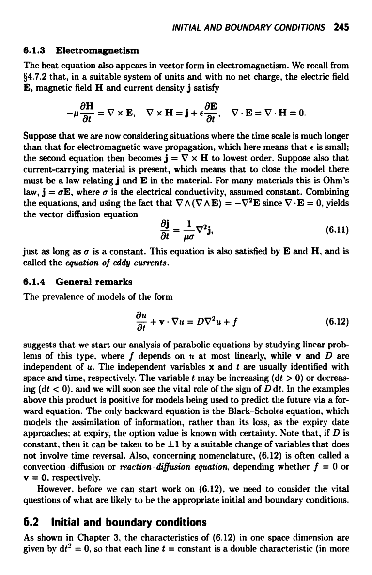
We now make three important modelling assumptions. The first is that the instan-

taneous 'rate of return' on the asset varies randomly, so that

µ dt + or dX, (6.9)

where p is a deterministic 'growth rate' for the asset; more importantly, dX is a

small normal random variable102 of mean zero and variance dt which models the

uncertain response of the share price to the arrival of new information, and a is a

parameter which measures how 'volatile' the share price is. We can estimate the

change in V = V(S, t) in a time interval dt by writing

dV =

dt +

ds + 2852 (dS)2 + .

Now dS is given by (6.9), and we take the second bold step of assuming that

the largest contribution to dS2 is a2S2 dX2 and then replacing dX2 by dt, since

X has zero mean and variance dt. This second step is equivalent to the assumption

that is needed to go from (6.7) to (6.8), namely k2 = 0(h), and it can be described

systematically using Ito's lemma from stochastic calculus [31]. The upshot is that

dS +

10_2S2

8SV2 dt + o(dt).

dP = rM dt + A dS +

dt +

This enables us to make the key observation that we can instantaneously remove

all the randomness, represented by dS, from our portfolio by choosing A to be

-ay/as.

The final step is to use the idea of no arbitrage, which is the technical term for

the non-existence of a 'free lunch'. In this context, it means that it is impossible to

earn more than the risk-free interest rate r for a risk-free portfolio, so dP = rP dt

and hence we derive the Black-Scholes equation

2a2S2S2

= r

-Sas) (6.10)

for the value of our option. Note that, as compared toll

the heat equation, the

Black-Scholes equation is a 'backward' parabolic equation with a convective term

rS OV/aS and a 'source' term rV, and we expect intuitively that a final condition

should be imposed. This is that V equals S - E at t = T, provided that S > E,

which represents the proceeds of exercising the option and immediately selling the

asset; if, on the other hand, S < E, the holder will not wish to pay more for the

asset than it is worth, and in this case the option is not exercised, so V = 0. We

note that if S vanishes at some time it remains zero, according to (6.9), so the

boundary condition V = 0 at S = 0 must also hold.103

'°2There have been many more large swings in world markets than would be consistent with

the assumption of a normal random variable; this model must be used with caution!

103Tho discussion we have given is just the starting point of an enormous range of valuation

problems for 'vanilla' and 'exotic' options in the Black-Scholes framework; most of them are

boundary value problems for the Black-Scholes equation or a variant of it, and we refer the

reader to [47[.

INITIAL AND BOUNDARY CONDITIONS 245

6.1.3 Electromagnetism

The heat equation also appears in vector form in electromagnetism. We recall from

§4.7.2 that, in a suitable system of units and with no net charge, the electric field

E, magnetic field H and current density j satisfy

-µaH=VxE,

VxH=j+eBE,

Suppose that we are now considering situations where the time scale is much longer

than that for electromagnetic wave propagation, which here means that a is small;

the second equation then becomes j = V x H to lowest order. Suppose also that

current-carrying material is present, which means that to close the model there

must be a law relating j and E in the material. For many materials this is Ohm's

law, j = aE, where a is the electrical conductivity, assumed constant. Combining

the equations, and using the fact that V A (V A E) = -O2E since V E = 0, yields

the vector diffusion equation

_ 1

V j, (6.11)

just as long as a is a constant. This equation is also satisfied by E and H, and is

called the equation of eddy currents.

6.1.4 General remarks

The prevalence of models of the form

(6.12)

suggests that we start our analysis of parabolic equations by studying linear prob-

lems of this type. where f depends on it at most linearly, while v and D are

independent of u. The independent variables x and t are usually identified with

space and time, respectively. The variable t may be increasing (dt > 0) or decreas-

ing (dt < 0), and we will soon see the vital role of the sign of D dt. In the examples

above this product is positive for models being used to predict the future via a for-

ward equation. The only backward equation is the Black-Scholes equation, which

models the assimilation of information, rather than its loss, as the expiry date

approaches; at expiry, the option value is known with certainty. Note that, if D is

constant, then it can be taken to be ±1 by a suitable change of variables that does

not involve time reversal. Also, concerning nomenclature, (6.12) is often called a

convection -diffusion or reaction-diffusion equation, depending whether f = 0 or

v = 0, respectively.

However, before we can start work on (6.12). we need to consider the vital

questions of what are likely to be the appropriate initial and boundary conditions.

6.2 Initial and boundary conditions

As shown in Chapter 3, the characteristics of (6.12) in one space dimension are

given by dt2 = 0, so that each line t = constant is a double characteristic (in more

246

PARABOLIC EQUATIONS

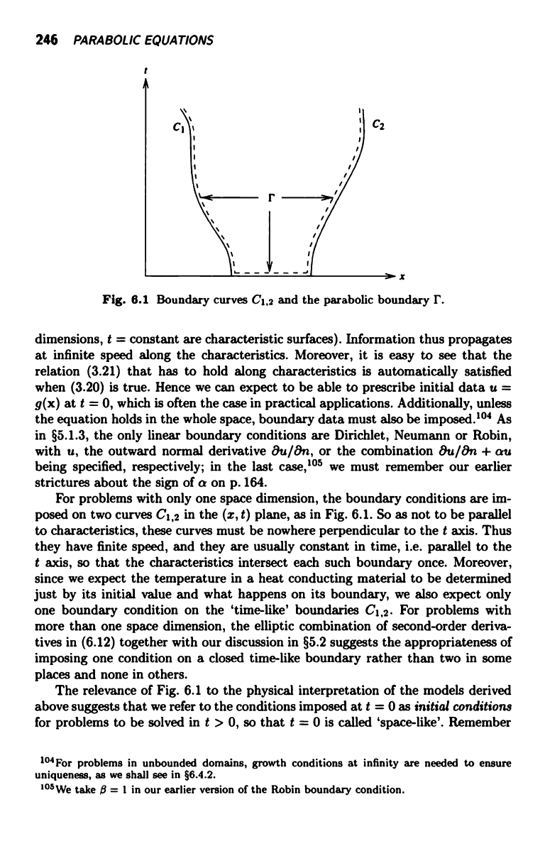
Fig. 6.1 Boundary curves C1,2 and the parabolic boundary I'.

dimensions, t = constant are characteristic surfaces). Information thus propagates

at infinite speed along the characteristics. Moreover, it is easy to see that the

relation (3.21) that has to hold along characteristics is automatically satisfied

when (3.20) is true. Hence we can expect to be able to prescribe initial data u =

g(x) at t = 0, which is often the case in practical applications. Additionally, unless

the equation holds in the whole space, boundary data must also be imposed. 10" As

in §5.1.3, the only linear boundary conditions are Dirichlet, Neumann or Robin,

with u, the outward normal derivative 8u/8n, or the combination Ou/8n + au

being specified, respectively; in the last case,105 we must remember our earlier

strictures about the sign of a on p. 164.

For problems with only one space dimension, the boundary conditions are im-

posed on two curves C1,2 in the (x, t) plane, as in Fig. 6.1. So as not to be parallel

to characteristics, these curves must be nowhere perpendicular to the t axis. Thus

they have finite speed, and they are usually constant in time, i.e. parallel to the

t axis, so that the characteristics intersect each such boundary once. Moreover,

since we expect the temperature in a heat conducting material to be determined

just by its initial value and what happens on its boundary, we also expect only

one boundary condition on the 'time-like' boundaries C1,2. For problems with

more than one space dimension, the elliptic combination of second-order deriva-

tives in (6.12) together with our discussion in §5.2 suggests the appropriateness of

imposing one condition on a closed time-like boundary rather than two in some

places and none in others.

The relevance of Fig. 6.1 to the physical interpretation of the models derived

above suggests that we refer to the conditions imposed at t = 0 as initial conditions

for problems to be solved in t > 0, so that t = 0 is called 'space-like'. Remember

104 For problems in unbounded domains, growth conditions at infinity are needed to ensure

uniqueness, as we shall see in §6.4.2.

105We take 6 = I in our earlier version of the Robin boundary condition.

MAXIMUM PRINCIPLES AND WELL-POSEDNESS 247

that the first example of §3.1 confirms that one initial condition should be given

rather than one `final' one. This is also apparent from considering the limiting

procedure of obtaining the heat equation from the hyperbolic equation

282u 8u 02u

8t2 + 8t = 8x2

as a -> 0, where the argument of §3.4.3 also suggests that when D dt > 0 only one

initial condition should be imposed at t = 0.

There are many methods for proving existence and uniqueness results for

parabolic equations, most of which are too abstract for this book. As in the pre-

vious two chapters, we will mostly be concerned, especially in §§6.4 and 6.5, with

explicit representations of solutions, so that the existence question will not arise.

However, the maximum principle is such a generally applicable tool for proving

uniqueness that we will begin by describing its use in §6.3, before going on to

describe techniques used to obtain explicit solutions to linear equations in integral

and series form. Another way of obtaining special solutions that has only received

brief attention in Chapters 4 and 5 is that of reducing the number of independent

variables through invariance properties. We consider this in some detail in §6.5,

before applying it to nonlinear equations in §6.6, where other methods suitable for

studying such equations are also reviewed. The final section takes a quick look at

some second-order parabolic systems and higher-order parabolic equations.

6.3

Maximum principles and well-posedness

Even more than in the elliptic case, the idea of maximum principles is invaluable

in assessing well-posedness properties of parabolic equations. Parabolic maximum

principles, like those of the preceding chapter, apply in any number of space di-

mensions. The maximum principle for the simplest inhomogeneous heat equation

states that, if

Ou = V2u

+ f (X, t)

and f < 0, then u takes its maximum on the parabolic boundary, denoted by r,

where the initial and boundary conditions are given (see Fig. 6.1). Thus, when the

equation holds for x in it and 0 < t < T, u is largest either on 8fl or at t = 0. This

is of course what we expect physically. If heat is being lost through a volumetric

heat sink with f < 0, then heat flows into 0 from the boundary and is removed in

the interior, and the maximum temperature must be on the boundary if it is not

at t = 0; equally, with f > 0, u takes its minimum on the parabolic boundary.

The proof is similar to that for the maximum principle for Laplace's equation

in §5.3. Consider first f < 0; then, at an interior maximum 8u/8t = 0, Vu = 0

and V2u < 0, leading to a contradiction. For a maximum on t = T, 8u/8t 0,

Vu = 0 and V2u < 0, again leading to a contradiction, so the maximum must lie

on F. To consider f < 0, write v = u +

elx12/2m, taking

m to be the number of

space dimensions. Then

8v 2

8t_pv=f-E<0,