Novak P. Developments in hydraulic engineering

Подождите немного. Документ загружается.

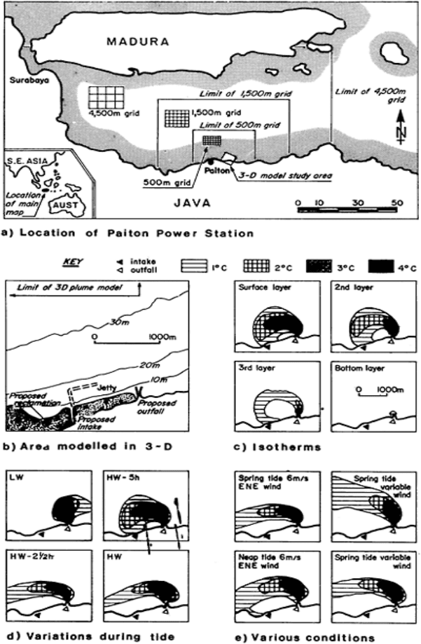
FIG. 5. Paiton power station;

hydrodynamic modelling using

Distributed Array Processors.

(Courtesy of Hydraulics Research

Ltd.)

The interface between estuaries and seas 149

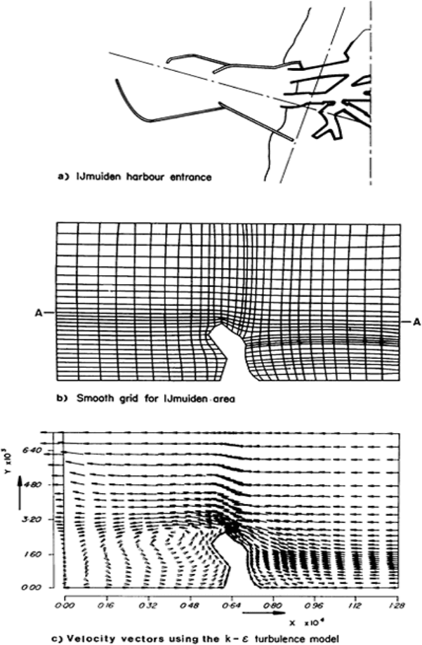
FIG. 6. Flow conditions outside

Ijmuiden harbour, computed using

model ODYSEE. (Based on reference

49, figures 19, 22 and 24, by courtesy

of Pineridge Press, Swansea.)

Developments in hydraulic engineering–5 150

generate curvilinear coordinates from depth contours. This has proved useful for study of

small areas over which spatial changes of surface elevation can be neglected. Because the

curvilinear grid is depth-generated, the depth cannot vary with time. This can be achieved

in tidal situations by assuming a rigid lid as the upper boundary and specifying a free slip

condition there. The effect of rise and fall of surface can be partially simulated by

allowing pressures on the underside of the imaginary lid to vary. Figure 6 shows

application of a rigid-lid model to Ijmuiden harbour entrance; Fig. 6(b) shows the

computer-generated grid while Fig. 6(c) shows computed velocity vectors.

The choice of modelling method depends on the problems being studied. Numerical

modelling specialists have a range of options available to them and combine them to

achieve the best results at acceptable cost. It is possible to use a coarse rectangular grid

for a regional model, and a stretched or curvilinear grid for local studies. The equations

can be solved using fractional time steps as described in Section 6.

Implicit modelling

methods have been used very widely, largely because of their inherent stability when

using relatively large time steps. Their accuracy has been improved by various means.

However, as more interacting phenomena are introduced, the equations become

increasingly complicated and the advantages compared with explicit schemes diminish.

Distributed array processors are very useful for complicated conditions. They can only be

used with explicit methods, which are potentially more accurate than implicit when

stability criteria are satisfied.

7 REGIONAL MODELLING OF WAVES

7.1 Modelling Methods

There are several well tried models which can be used to predict the ‘global’ wave

climate in deep water at the boundaries of the region being studied.

They are beyond the

scope of this chapter.

The primary objective of modelling waves is to determine the local climate of waves

and currents so that sediment movements or dispersion of pollutants can be analysed. To

this end, it is necessary to know the directional spectra of waves propagating into or

through the region and to (i) analyse their modification by shallow water, friction and

breaking, (ii) estimate the pattern of wave-induced currents, and (iii) analyse their

interaction with tidal and river currents.

Solution of the full equations is difficult and would be prohibitively expensive if

applied over an area typical of an outer estuary. Various compromises are necessary in

order to reach engineering solutions. One is to divide the modelled area into regions in

each of which different simplifying assumptions can be made. It is convenient to consider

an outer and an inner region. In the outer region refraction is assumed to be the most

important effect. Weak diffraction may also occur. The inner region includes refraction of

waves by currents, all breaking waves and regions inshore of them, and thus includes the

effects of radiation stresses and wave-induced currents. It is also the region of greatest

rates of sediment transport. Some modelling methods bridge these regions but, for

convenience, the outer region is discussed in this section while the inner region is

considered in Section 8.

The interface between estuaries and seas 151

Four methods of modelling surface waves in transitional and shallow-water depths

have been used.

(1) The most general approach is to obtain solutions to the wave equations of

momentum and continuity in terms of surface elevation and particle velocity throughout

the whole domain of interest at a particular time, and then to advance the solution in a

series of time steps. This is necessarily extremely expensive in computer time, and

simplifications must be made before it can be used even for small areas such as inside

harbours. Practical economies can be made in suitable cases by using the Boussinesq

equations, which apply to finite-amplitude waves with irrotational motion in inviscid

water over a horizontal bed. Reasonable accuracy can be achieved at small values of

depth/wavelength (<0.15),

but the range of application can be increased by including

higher-order terms in the difference equations.

(2) If the wave climate changes only slowly with time, and linear theory is acceptable

(small wave height), a steady-state harmonic solution for surface elevations and velocities

can be assumed. The wave equation for this case is elliptical in form and must be treated

as a boundary-value problem. It can include the effect of multiple reflections, refraction

and diffraction. Possible solution methods are finite differences and finite elements. This

model is only suitable for limited areas due to the high cost of computation, but requires

less computing effort than solution of the Boussinesq equations.

(3) Further simplification can be made if the effects of wave reflections are excluded

from the solution. In that case, the equation can be approximated by one of parabolic

form which can be solved as a problem of propagation, using a marching solution from

the seaward boundary.

This results in considerable economies over elliptical-equation

models.

These three modelling methods require computations to be done on a grid fine enough

to resolve wave height over each wavelength—preferably at least 10 points, though fewer

have been used. The grid spacing is typically 5–10 m.

(4) The fourth method is the ray method, based on geometrical optical theory. It is

assumed that, in the absence of currents, waves propagate along orthogonals or rays and

that energy is conserved between orthogonals. An initial-value problem can then be

solved along each ray. The only inputs needed for monochromatic waves are period and

water depth, and computation need only be done at intervals close enough to resolve

significant changes in depth, typically of order 200 m. This method allows changes in

concentration of energy flux to be calculated so that changes in relative wave height can

be deduced using small-amplitude theory. The basic method does not allow diffraction or

reflections to be taken into account.

Each of these four general approaches has been developed so that different effects can

be modelled. Variations of these methods have also been devised so that refraction of

waves by depth and current changes can be studied.

7.2 Modelling Wave Refraction

The classic approach to study of wave propagation towards coasts was to apply simple

refraction theory to discrete components of a wave spectrum and to build up as complete

a picture as possible within available time and cost (e.g. Munk and Arthur

). Refraction

occurs when wave propagation speed is changed locally as a consequence of changes in

Developments in hydraulic engineering–5 152

water depth. Small-amplitude wave propagation is governed by the linear dispersion

equation ω

=gk tanh kd, from which wave propagation speed is c=ω/k and wave group

velocity is

ω is angular wave frequency=2π/T; T is wave period; k is wave number=2π/L where L is

wavelength; d is mean water depth over a wave period. Wave rays can be determined for

monochromatic waves of small amplitude. An approximation to real wave behaviour can

be made by assuming that a spectrum consists of a number of discrete components that

can be added linearly.

Bottom topography can cause wave rays to converge or diverge with resultant increase

or decrease in energy flux per unit width. If rays converge to coincidence they form

‘caustic’ curves which indicate that theoretical energy flux per unit width becomes

infinite. In reality, wave diffraction would occur and some wave energy would be

dissipated by friction and breaking before reaching a predicted region of caustics.

Modelling of simple refraction, e.g. by developing wave rays, is a very economical

method because it does not require computation of wave profiles; it depends only on

knowledge of local water depths. However, the assumption of linear superposition of

discrete spectral components breaks down when steep finite waves occur and when

waves approach regions of caustics. Development of wave rays is Lagrangian in form and

is not a convenient method for computation of interaction of waves with tidal currents

and of sediment transport.

The wave ray method can be adapted to an Eulerian form by using a finite difference

method based on a fixed grid and computing wave properties at grid points by

interpolation. By excluding diffraction from the analysis, wave phase and wave energy

can be decoupled; this is, essentially, a feature of the wave ray method. Non-linear

bottom friction and energy losses due to wave breaking can be included in such a model.

Grid spacing is not critical to the analysis, the only requirement being that bottom

topography should be adequately modelled. A grid spacing of 200 m or more is usually

satisfactory. Using such a model, Sakai et al.

considered the propagation of spectral

wave components from discrete directions at one fixed frequency. Booij et al.

developed a similar model to include changes in that frequency and associated changes in

energy density. The alternative of choosing several frequencies, each with its energy

concentrated in one particular direction, was developed by Chen and Wang.

A further

development which includes diffraction, due to Yoo and O’Connor,

is described below.

7.3 Modelling Both Diffraction and Refraction

To deal with the problem of wave propagation over a rapidly varying topography,

modelling of both refraction and diffraction is needed. Early models for diffraction were

restricted to water of constant mean depth.

No refraction can occur under such

conditions. Combined refraction and diffraction can be studied in models in which the

wave equation is solved in two dimensions in plan.

The space-time grid must be fine

enough to allow the wave profiles to be resolved adequately (5–10 m), yet the areas to be

modelled must include extensive regions of shallow water. Such models are extremely

expensive to operate, and their practical use is restricted to local regions where

The interface between estuaries and seas 153

appreciable gradients of wave energy have been predicted by simple refraction models. In

real situations, waves and currents have large random components which add to the

complexity of analysis. Practical models must have limited objectives. There are many

alternatives and the final choice will depend on the particular problem to alternatives and

the final choice will depend on the particular problem to be solved. Models which can

only provide steady-state solutions can be accepted if the real situation varies only slowly

in its overall behaviour. Harmonic solutions may have to be accepted if their adoption

results in very large savings in computer effort.

7.4 The ‘Mild-slope’ Equation

One compromise is to limit the model to gradually-varying bottom topography. The basis

of this method is the ‘mild-slope’ equation first derived by Berkhoff.

It is elliptic in

form. Valid solutions of this equation must be harmonic and steady-state.

Considerable

economies in computation can be made if the equation can be modified to a parabolic

form. This was done by Radder

and Booij

to include interaction with non-uniform

currents (in plan) and energy dissipation effects due to wave breaking and bottom

friction. Their version is valid for transient and non-harmonic solutions but it is only

valid for progressive waves and cannot be used when there are strong wave reflections.

A full derivation of the mild-slope equation in various forms is given by Copeland.

is based on conservation of wave energy, which requires that the rate of change of wave

energy equals the rate at which work is done by external pressure:

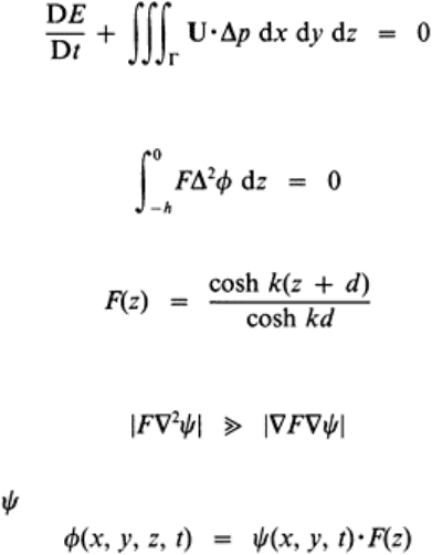
(11)

where E is wave energy per unit area; ∆=∂/∂x, ∂/∂y, ∂/∂z; Γ represents a control volume.

Equation (11) leads to

(12)

where

(13)

Two important conditions are imposed: (1) energy is conserved; (2) the bed must be

mildly sloping, such that

(14)

where

is velocity potential at z=0. The velocity potential

(15)

Equation (14) leads to

Developments in hydraulic engineering–5 154

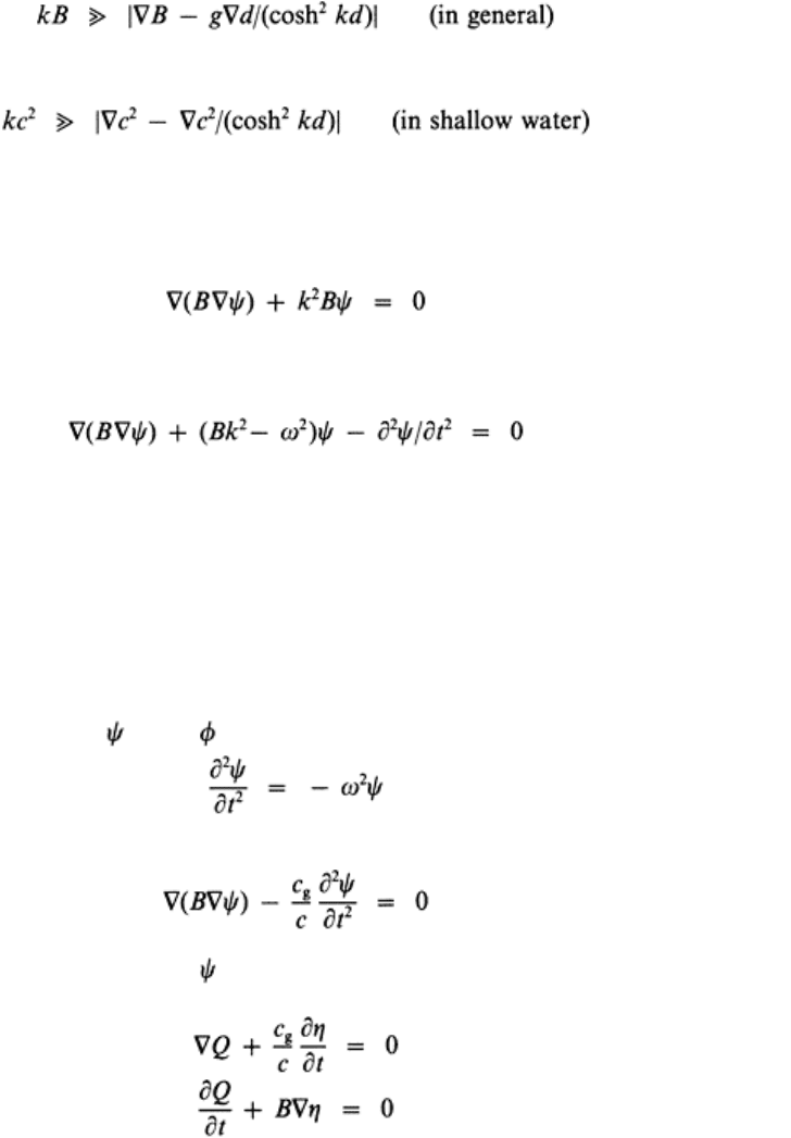
(16)

where B=c·c

, or

(17)

which imply that there must not be appreciable changes in depth over the length of a

wave.

In its steady-state, harmonic form the mild-slope equation due to Berkhoff

and

modified by Smith and Spinks

and Lozano and Meyer

may be written

(18)

This is an elliptic equation which can be solved as a boundary value problem. In its

transient form without currents it may be written

11,15,16

(19)

Note that the mild-slope equation, in all its forms, is for monochromatic waves. The

parabolic approximation only applies to waves with directions nearly collinear with one

of the coordinate axes. Wave spectra and their modification cannot be reproduced

directly, and the method breaks down if the waves undergo marked changes in direction

as in the lee of islands, shoals or breakwaters. Parabolic solutions of the mild-slope

equation have been based on the assumption of progressive waves. They do not apply to

regions where there are strong wave reflections.

In order to overcome some of these deficiencies, Copeland

15,16

modified the mild-

slope equation to a hyperbolic form. The steady-state harmonic form of the velocity

potential is

(x, y, t)= (x, y)exp(−iωt). From this,

(20)

Inserting this in eqn. (18) leads to

(21)

The surface condition

=−i(g/ω)η gives

This hyperbolic equation can be expressed as two first-order equations:

(23)

(24)

The interface between estuaries and seas 155

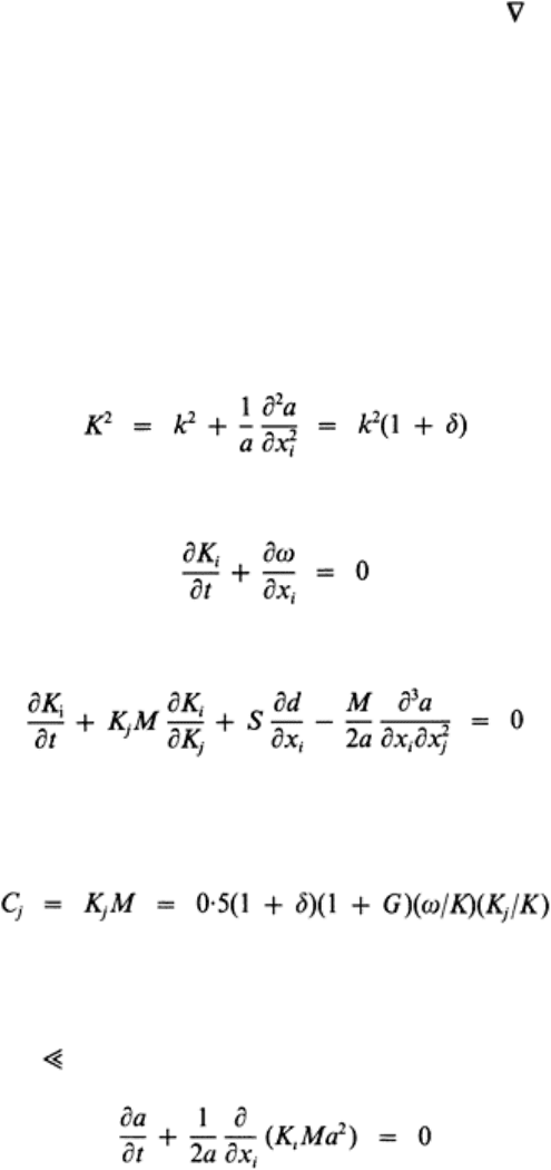
where Q is a dummy variable. It is harmonic in form, but its physical form is only needed

on the model boundaries. Q=c

η is a solution provided that c

=0.

This is therefore useful in deep water or in water of constant depth. It can be

calculated at model boundaries, provided only that depth at these boundaries is locally

constant. Reflections can be included and, as there is no constraint on wave direction, it

can be used down-wave of islands, shoals and breakwaters. The periodic solution of eqns

(23) and (24) travels with phase speed given by c

=(g/k)tanh(kd), which implies

conservation of wave action. There is no restriction on depth of water.

7.5 Analysis of Diffraction Using Wave Rays

Yoo and O’Connor

used a development of ray theory which has higher computational

efficiency because it is based on wave dispersion rates rather than on detailed knowledge

of wave profiles. The small-amplitude dispersion relationship is ω

=gktanh(kd). Battjes

had shown that, when diffraction occurs, the separation factor k should be replaced by

wave number K:

(25)

where i,j=1,2 (coordinate directions in plan), and a is wave amplitude.

Using this relationship in conjunction with the kinematic equation

(26)

Yoo and O’Connor obtained a wave crest conservation equation applicable to caustic or

diffractive gravity waves:

(27)

where M=0·5(1+G)(ω/k)(1/k); S=ωG/(2d); G=2kd/(sinh 2kd); d is total water depth=h+η;

h is still water depth (including tidal rise and fall); η is mean surface elevation over a

wave period.

The group velocity of caustic waves is

(28)

Equation (28) reduces to ordinary linear wave theory when δ=0.

The Battjes relation, eqn (25), also influences dynamic wave motion when diffraction

occurs. Yoo

has shown that its effect is small and can be neglected when caustics are

mild (δ

1). When dissipation effects are small, dynamic conservation of waves is given

(29)

Developments in hydraulic engineering–5 156

Yoo developed a numerical scheme for solution of these equations and compared its

predictions with experimental results obtained by Ito and Tanimoto

for the case of a

circular shoal which generated caustics when studied by simple ray theory. He also

applied it to experimental results obtained by Berkhoff for a case of refraction and

diffraction around twin ellipsoidal shoals, with good results.

8 MODELLING OF NEARSHORE WAVES AND CURRENTS

8.1 Introduction

At the sea-face of estuaries, wave action on terminal bars and sandbanks greatly enhances

sediment transport due to tidal currents. In the major ebb- and flood-dominated channels,

wave action at the bed is weaker but tidal currents are strong. There is a complicated

pattern of sediment movement in the region, which varies according to the states of tide,

wave action and fresh water discharge. Bed forms and, consequently, bed resistance

undergo frequent change. At present there is little knowledge of bed forms caused by

oscillatory flows combined with currents at an arbitrary angle though some

measurements have been made in particular cases. This limits the potential accuracy of

computation of local currents and wave action. Wave action causes radiation stresses

which cause wave-induced currents, particularly near to and inshore of the breaker zone.

In some cases, waves break on outer bars and re-form inshore of them. Knowledge of

wave behaviour after breaking is still largely empirical. All these effects can be

reproduced, but not in any one model. There is a range of models available, each of

which can reproduce some aspects of the whole situation quite well. In breaking down a

problem into several components, it has to be assumed that each behaves independently.

This is not correct, and care has to be taken to ensure that the final result is a sufficient

representation of reality for the purpose.

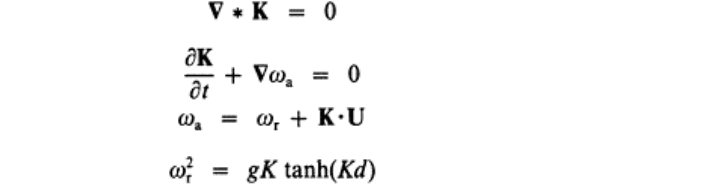
8.2 Wave/Current Interactions

In the nearshore region, wave breaking and wave-induced currents must be accounted for.

Wave interactions with tidal currents can also be important.

26,32,33

To account for the

effects of combined waves and currents, it is necessary to consider the motion of waves

relative to the body of moving water as well as the absolute celerity of the waves. Calling

the angular frequencies ω

and ω

respectively, the equations for interaction are

(30)

(31)

(32)

(33)

The interface between estuaries and seas 157

where K is wave number, d is water depth, and U is depth-mean velocity. Symbols in

bold type represent vectors, * indicates vector product, and • scalar product. d includes

the set-up or set-down of mean water level from tidal water level.

8.3 Solutions Based on the ‘Mild-slope’ Equation and Related

Methods

One family of methods of modelling waves and currents is based on the mild-slope

equation in its steady-state form, eqn (18), or its transient form, eqn (19). When tidal

currents can be neglected, eqns (23) and (24) can be used. Once eqns (23) and (24) have

been solved for a particular situation, radiation stresses can be calculated and used to

estimate wave-induced currents which can be calculated with the aid of a steady-flow

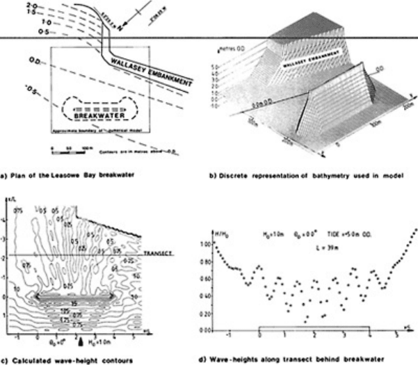
model. Copeland used this method to analyse wave set-up and wave-induced currents

around an offshore breakwater in Liverpool Bay. In the form published by Copeland,

this model does not reproduce the effects of wave interaction with tidal currents.

FIG. 7. Wave conditions at Leasowe

bay computed using Copeland’s

model. (Based on reference 15, figures

9.61 (a) and (b) and 9.62 (a) and (b),

by courtesy of Dr G.Copeland.)

Developments in hydraulic engineering–5 158

Novak P. Developments in hydraulic engineering - Vol. 5

Подождите немного. Документ загружается.