Nigel S., Chambers S., Johnson R. Operations Management

Подождите немного. Документ загружается.

Johnson’s rule

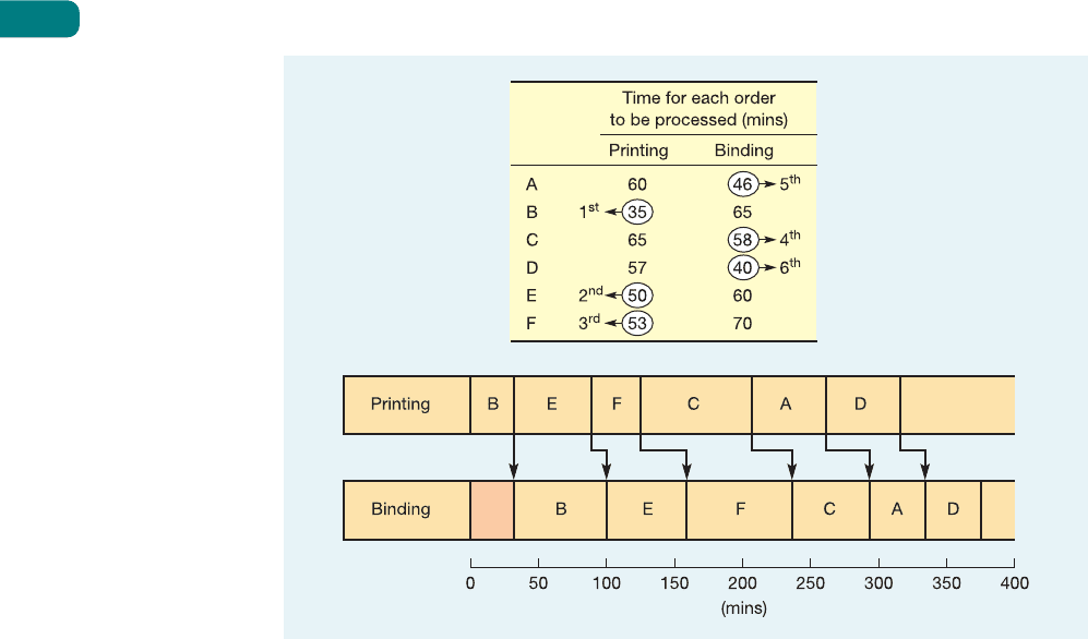
Johnson’s rule applies to the sequencing of n jobs through two work centres. Figure 10.9

illustrates its use. In this case, a printer has to print and bind six jobs. The times for process-

ing each job through the ﬁrst (printing) and second (binding) work centres are shown in

the ﬁgure. The rule is simple. First look for the smallest processing time. If that time is

associated with the ﬁrst work centre (printing in this case) then schedule that job ﬁrst, or

as near ﬁrst as possible. If the next smallest time is associated with the second work centre

then sequence that job last or as near last as possible. Once a job has been sequenced, delete

it from the list. Carry on allocating jobs until the list is complete. In this particular case,

the smallest processing time is 35 minutes for printing job B. Because this is at the ﬁrst pro-

cess (printing), job B is assigned ﬁrst position in the schedule. The next smallest processing

time is 40 minutes for binding (job D). Because this is at the second process (binding), it is

sequenced last. The next lowest processing time, after jobs B and D have been struck off the

list, is 46 minutes for binding job A. Because this is at the second work centre, it is sequenced

as near last as possible, which in this case is ﬁfth. This process continues until all the jobs

have been sequenced. It results in a schedule for the two processes which is also shown in

Figure 10.9.

Scheduling

Having determined the sequence that work is to be tackled in, some operations require

a detailed timetable showing at what time or date jobs should start and when they should end

– this is scheduling. Schedules are familiar statements of volume and timing in many con-

sumer environments. For example, a bus schedule shows that more buses are put on routes

at more frequent intervals during rush-hour periods. The bus schedule shows the time each

bus is due to arrive at each stage of the route. Schedules of work are used in operations where

some planning is required to ensure that customer demand is met. Other operations, such

Part Three Planning and control

284

Johnson’s rule

Scheduling

Figure 10.9 The application of Johnson’s rule for scheduling n jobs through two work

centres

M10_SLAC0460_06_SE_C10.QXD 10/20/09 9:33 Page 284

as rapid-response service operations where customers arrive in an unplanned way, cannot

schedule the operation in a short-term sense. They can only respond at the time demand is

placed upon them.

The complexity of scheduling

The scheduling activity is one of the most complex tasks in operations management. First,

schedulers must deal with several different types of resource simultaneously. Machines will

have different capabilities and capacities; staff will have different skills. More importantly,

the number of possible schedules increases rapidly as the number of activities and processes

increases. For example, suppose one machine has ﬁve different jobs to process. Any of the

ﬁve jobs could be processed ﬁrst and, following that, any one of the remaining four jobs,

and so on. This means that there are:

5 × 4 × 3 × 2 = 120 different schedules possible

More generally, for n jobs there are n! (factorial n) different ways of scheduling the jobs

through a single process.

We can now consider what impact there would be if, in the same situation, there was

more than one type of machine. If we were trying to minimize the number of set-ups on

two machines, there is no reason why the sequence on machine 1 would be the same as the

sequence on machine 2. If we consider the two sequencing tasks to be independent of each

other, for two machines there would be

120 × 120 = 14,400 possible schedules of the two machines and ﬁve jobs.

A general formula can be devised to calculate the number of possible schedules in any

given situation, as follows:

Number of possible schedules = (n!)m

where n is the number of jobs and m is the number of machines.

In practical terms, this means that there are often many millions of feasible schedules,

even for relatively small operations. This is why scheduling rarely attempts to provide an

‘optimal’ solution but rather satisﬁes itself with an ‘acceptable’ feasible one.

Forward and backward scheduling

Forward scheduling involves starting work as soon as it arrives. Backward scheduling

involves starting jobs at the last possible moment to prevent them from being late. For exam-

ple, assume that it takes six hours for a contract laundry to wash, dry and press a batch of

overalls. If the work is collected at 8.00 am and is due to be picked up at 4.00 pm, there are

more than six hours available to do it. Table 10.3 shows the different start times of each job,

depending on whether they are forward- or backward-scheduled.

The choice of backward or forward scheduling depends largely upon the circumstances.

Table 10.4 lists some advantages and disadvantages of the two approaches. In theory, both

materials requirements planning (MRP, see the supplement to Chapter 14) and just-in-time

planning (JIT, see Chapter 15) use backward scheduling, only starting work when it is

required. In practice, however, users of MRP have tended to allow too long for each task to

be completed, and therefore each task is not started at the latest possible time. In comparison,

JIT is started, as the name suggests, just in time.

Chapter 10 The nature of planning and control

285

Table 10.3 The effects of forward and backward scheduling

Task Duration Start time (backwards) Start time (forwards)

Press 1 hour 3.00 pm 1.00 pm

Dry 2 hours 1.00 pm 11.00 am

Wash 3 hours 10.00 am 8.00 am

Forward scheduling

Backward scheduling

M10_SLAC0460_06_SE_C10.QXD 10/20/09 9:33 Page 285

Gantt charts

The most common method of scheduling is by use of the Gantt chart. This is a simple device

which represents time as a bar, or channel, on a chart. Often the charts themselves are made

up of long plastic channels into which coloured pieces of paper can be slotted to indicate

what is happening with a job or a work centre. The start and ﬁnish times for activities can

be indicated on the chart and sometimes the actual progress of the job is also indicated.

The advantages of Gantt charts are that they provide a simple visual representation both of

what should be happening and of what actually is happening in the operation. Furthermore,

they can be used to ‘test out’ alternative schedules. It is a relatively simple task to represent

alternative schedules (even if it is a far from simple task to ﬁnd a schedule which ﬁts all

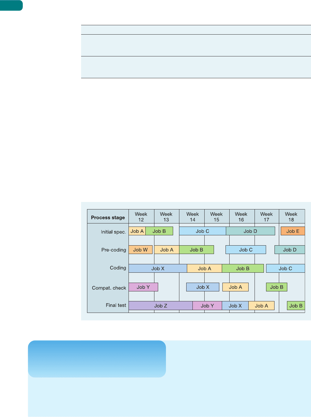
the resources satisfactorily). Figure 10.10 illustrates a Gantt chart for a specialist software

developer. It indicates the progress of several jobs as they are expected to progress through

ﬁve stages of the process. Gantt charts are not an optimizing tool, they merely facilitate the

development of alternative schedules by communicating them effectively.

Part Three Planning and control

286

Table 10.4 Advantages of forward and backward scheduling

Advantages of forward scheduling Advantages of backward scheduling

High labour utilization – workers Lower material costs – materials are not used until

always start work to keep busy they have to be, therefore delaying added value until

the last moment

Flexible – the time slack in the system Less exposed to risk in case of schedule change by

allows unexpected work to be loaded the customer

Tends to focus the operation on customer due dates

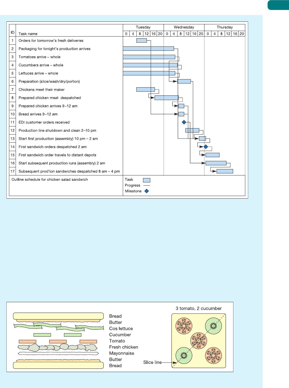
Pre-packed sandwiches are a growth product around the

world as consumers put convenience and speed above

relaxation and cost. But if you have recently consumed a

pre-packed sandwich, think about the schedule of events

Short case

The life and times of a chicken

salad sandwich – part one

which has gone into its making. For example, take a

chicken salad sandwich. Less than 5 days ago, the

chicken was on the farm unaware that it would never

see another weekend. The Gantt chart schedule shown

in Figure 10.11 tells the story of the sandwich, and

(posthumously), of the chicken.

From the forecast, orders for non-perishable items are

placed for goods to arrive up to a week in advance of

their use. Orders for perishable items will be placed daily,

a day or two before the items are required. Tomatoes,

Figure 10.10 Gantt chart showing the schedule for jobs at each process stage

M10_SLAC0460_06_SE_C10.QXD 10/20/09 9:33 Page 286

Chapter 10 The nature of planning and control

287

cucumbers and lettuces have a three-day shelf life so

may be received up to three days before production.

Stock is held on a strict ﬁrst-in-ﬁrst-out (FIFO) basis.

If today is (say) Wednesday, vegetables are processed

that have been received during the last three days.

This morning the bread arrived from a local bakery and

the chicken arrived fresh, cooked and in strips ready

to be placed directly in the sandwich during assembly.

Yesterday (Tuesday) it had been killed, cooked, prepared

and sent on its journey to the factory. By midday orders

for tonight’s production will have been received on the

Internet. From 2.00 pm until 10.00 pm the production

Figure 10.11 Simpliﬁed schedule for the manufacture and delivery of a chicken salad sandwich

lines are closed down for maintenance and a very

thorough cleaning. During this time the production

planning team is busy planning the night’s production

run. Production for delivery to customers furthest

away from the factory will have to be scheduled ﬁrst.

By 10 pm production is ready to start. Sandwiches are

made on production lines. The bread is loaded onto a

conveyor belt by hand and butter is spread automatically

by a machine. Next the various ﬁllings are applied at

each stage according to the speciﬁed sandwich ‘design’,

see Figure 10.12. After the ﬁlling has been assembled

the top slice of bread is placed on the sandwich and

Figure 10.12 Design for a chicken salad sandwich

➔

M10_SLAC0460_06_SE_C10.QXD 10/20/09 9:33 Page 287

Scheduling work patterns

Where the dominant resource in an operation is its staff, then the schedule of work times

effectively determines the capacity of the operation itself. The main task of scheduling, there-

fore, is to make sure that sufﬁcient numbers of people are working at any point in time to

provide a capacity appropriate for the level of demand at that point in time. This is often called

staff rostering. Operations such as call centres, postal delivery, policing, holiday couriers, retail

shops and hospitals will all need to schedule the working hours of their staff with demand in

mind. This is a direct consequence of these operations having relatively high ‘visibility’ (we

introduced this idea in Chapter 1). Such operations cannot store their outputs in inventories

and so must respond directly to customer demand. For example, Figure 10.13 shows the

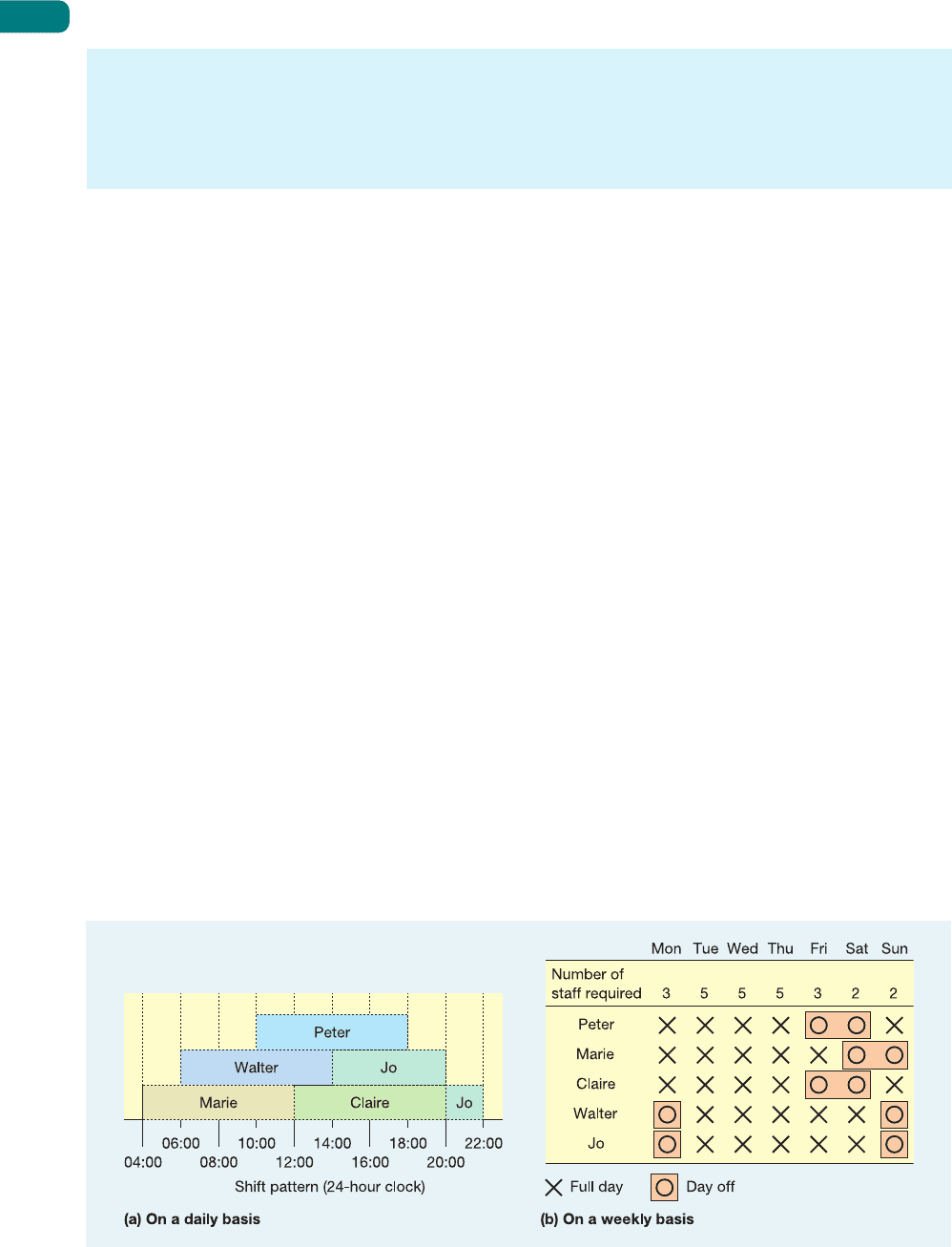
scheduling of shifts for a small technical ‘hot line’ support service for a small software company.

It gives advice to customers on their technical problems. Its service times are 4.00 hrs to 20.00

hrs on Monday, 4.00 hrs to 22.00 hrs Tuesday to Friday, 6.00 hrs to 22.00 hrs on Saturday,

and 10.00 hrs to 20.00 hrs on Sunday. Demand is heaviest Tuesday to Thursday, starts to

decrease on Friday, is low over the weekend and starts to increase again on Monday.

The scheduling task for this kind of problem can be considered over different timescales,

two of which are shown in Figure 10.13. During the day, working hours need to be agreed

with individual staff members. During the week, days off need to be agreed. During the year,

vacations, training periods and other blocks of time where staff are unavailable need to be

agreed. All this has to be scheduled such that:

● capacity matches demand;

● the length of each shift is neither excessively long nor too short to be attractive to staff;

● working at unsocial hours is minimized;

● days off match agreed staff conditions (for example) in this example – staff prefer two

consecutive days off every week;

● vacation and other ‘time-off’ blocks are accommodated;

● sufﬁcient ﬂexibility is built into the schedule to cover for unexpected changes in supply

(staff illness) and demand (surge in customer calls).

Part Three Planning and control

288

Figure 10.13 Shift scheduling in a home-banking enquiry service

machine-chopped into two triangles, packed and sealed

by machine. It is now early Thursday morning and by

2.00 am the ﬁrst refrigerated lorries are already departing

on their journeys to various customers. Production

continues through until 2.00 pm on the Thursday, after

which once again the maintenance and cleaning teams

move in. The last sandwiches are dispatched by 4.00 pm

on the Thursday. There is no ﬁnished goods stock.

Part two of the life and times of a chicken salad

sandwich is in Chapter 14.

Rostering

M10_SLAC0460_06_SE_C10.QXD 10/20/09 9:33 Page 288

Scheduling staff times is one of the most complex of scheduling problems. In the relatively

simple example shown in Figure 10.13 we have assumed that all staff have the same level

and type of skill. In very large operations with many types of skill to schedule and uncertain

demand (for example a large hospital) the scheduling problem becomes extremely complex.

Some mathematical techniques are available but most scheduling of this type is, in practice,

solved using heuristics (rules of thumb), some of which are incorporated into commercially

available software packages.

Monitoring and controlling the operation

Having created a plan for the operation through loading, sequencing and scheduling, each

part of the operation has to be monitored to ensure that planned activities are indeed

happening. Any deviation from the plans can then be rectiﬁed through some kind of inter-

vention in the operation, which itself will probably involve some replanning. Figure 10.14

illustrates a simple view of control. The output from a work centre is monitored and com-

pared with the plan which indicates what the work centre is supposed to be doing. Deviations

from this plan are taken into account through a replanning activity and the necessary inter-

ventions made to the work centre which will (hopefully) ensure that the new plan is carried

out. Eventually, however, some further deviation from planned activity will be detected and

the cycle is repeated.

Push and pull control

One element of control, then, is periodic intervention into the activities of the operation.

An important decision is how this intervention takes place. The key distinction is between

intervention signals which push work through the processes within the operation and those

which pull work only when it is required. In a push system of control, activities are scheduled

by means of a central system and completed in line with central instructions, such as an MRP

system (see Chapter 14). Each work centre pushes out work without considering whether the

succeeding work centre can make use of it. Work centres are coordinated by means of the

central operations planning and control system. In practice, however, there are many reasons

why actual conditions differ from those planned. As a consequence, idle time, inventory and

queues often characterize push systems. By contrast, in a pull system of control, the pace and

speciﬁcation of what is done are set by the ‘customer’ workstation, which ‘pulls’ work from

the preceding (supplier) workstation. The customer acts as the only ‘trigger’ for movement.

If a request is not passed back from the customer to the supplier, the supplier cannot produce

anything or move any materials. A request from a customer not only triggers production at the

supplying stage, but also prompts the supplying stage to request a further delivery from its

Chapter 10 The nature of planning and control

289

Push control

Pull control

Figure 10.14 A simple model of control

M10_SLAC0460_06_SE_C10.QXD 10/20/09 9:33 Page 289

own suppliers. In this way, demand is transmitted back through the stages from the original

point of demand by the original customer.

The inventory consequences of push and pull

Understanding the differing principles of push and pull is important because they have

different effects in terms of their propensities to accumulate inventory in the operation. Pull

systems are far less likely to result in inventory build-up and are therefore favoured by JIT

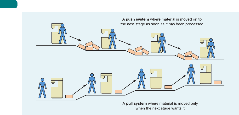
operations (see Chapter 15). To understand why this is so, consider an analogy: the ‘gravity’

analogy is illustrated in Figure 10.15. Here a push system is represented by an operation, each

stage of which is on a lower level than the previous stage. When parts are processed by each

stage, it pushes them down the slope to the next stage. Any delay or problem at that stage

will result in the parts accumulating as inventory. In the pull system, parts cannot naturally

ﬂow uphill, so they can only progress if the next stage along deliberately pulls them forward.

Under these circumstances, inventory cannot accumulate as easily.

Drum, buffer, rope

The drum, buffer, rope concept comes from the theory of constraints (TOC) and a concept

called optimized production technology (OPT) originally described by Eli Goldratt in his

novel The Goal.

(We will deal more with his ideas in Chapter 15.) It is an idea that helps to

decide exactly where in a process control should occur. Most do not have the same amount

of work loaded onto each separate work centre (that is, they are not perfectly balanced. This

means there is likely to be a part of the process which is acting as a bottleneck on the work

ﬂowing through the process. Goldratt argued that the bottleneck in the process should be

the control point of the whole process. It is called the drum because it sets the ‘beat’ for the

rest of the process to follow. Because it does not have sufﬁcient capacity, a bottleneck is

(or should be) working all the time. Therefore, it is sensible to keep a buffer of inventory

in front of it to make sure that it always has something to work on. Because it constrains

the output of the whole process, any time lost at the bottleneck will affect the output from

the whole process. So it is not worthwhile for the parts of the process before the bottleneck

to work to their full capacity. All they would do is produce work which would accumulate

further along in the process up to the point where the bottleneck is constraining the ﬂow.

Part Three Planning and control

290

Figure 10.15 Push versus pull: the gravity analogy

Drum, buffer, rope

Theory of constraints

M10_SLAC0460_06_SE_C10.QXD 10/20/09 9:33 Page 290

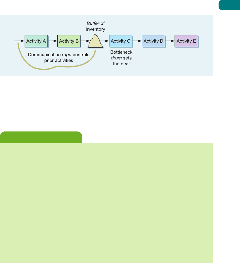
Therefore, some form of communication between the bottleneck and the input to the process

is needed to make sure that activities before the bottleneck do not overproduce. This is called

the rope (see Figure 10.16).

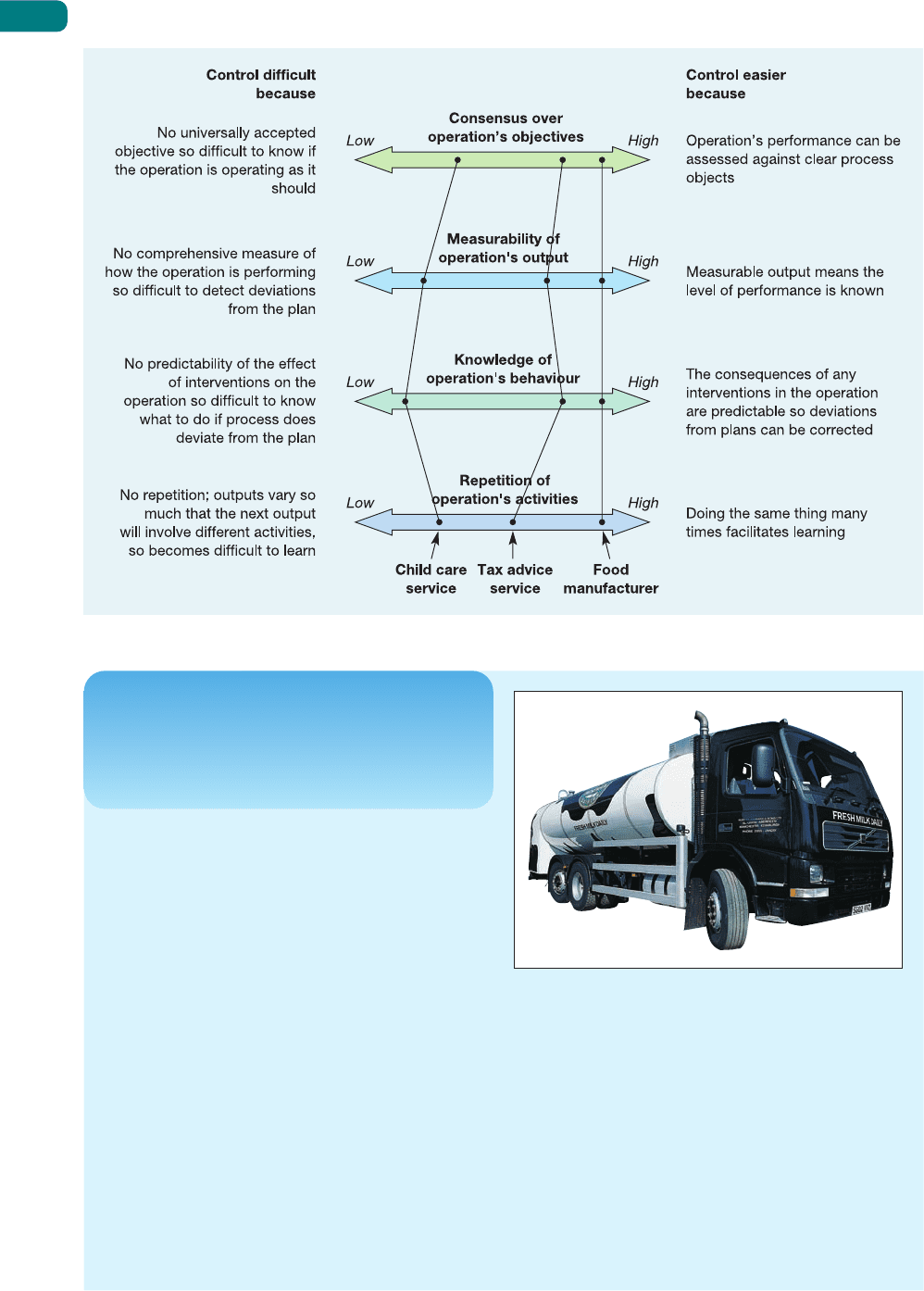
The degree of difﬁculty in controlling operations

The simple monitoring control model in Figure 10.15 helps us to understand the basic func-

tions of the monitoring and control activity. But, as the critical commentary box says, it is

a simpliﬁcation. Some simple technology-dominated processes may approximate to it, but

many other operations do not. In fact, the speciﬁc criticisms cited in the critical commentary

box provide a useful set of questions which can be used to assess the degree of difﬁculty

associated with control of any operation:

● Is there consensus over what the operation’s objectives should be?

● How well can the output from the operation be measured?

● Are the effects of interventions into the operation predictable?

● Are the operation’s activities largely repetitive?

Figure 10.17 illustrates how these four questions can form dimensions of ‘controllability’.

It shows three different operations. The food processing operation is relatively straightforward

to control, while the child care service is particularly difﬁcult. The tax advice service is some-

where in between.

Chapter 10 The nature of planning and control

291

Figure 10.16 The drum, buffer, rope concept

Most of the perspectives on control taken in this chapter are simpliﬁcations of a far more

messy reality. They are based on models used to understand mechanical systems such as

car engines. But anyone who has worked in real organizations knows that organizations

are not machines. They are social systems, full of complex and ambiguous interactions.

Simple models such as these assume that operations objectives are always clear and

agreed, yet organizations are political entities where different and often conﬂicting objectives

compete. Local government operations, for example, are overtly political. Furthermore,

the outputs from operations are not always easily measured. A university may be able to

measure the number and qualiﬁcations of its students, for example, but it cannot measure

the full impact of its education on their future happiness. Also, even if it is possible to

work out an appropriate intervention to bring an operation back into ‘control’, most

operations cannot perfectly predict what effect the intervention will have. Even the largest

of burger bar chains does not know exactly how a new shift allocation system will affect

performance. Also, some operations never do the same thing more than once anyway.

Most of the work done by construction operations is one-offs. If every output is different,

how can ‘controllers’ ever know what is supposed to happen? Their plans themselves are

mere speculation.

Critical commentary

M10_SLAC0460_06_SE_C10.QXD 10/20/09 9:33 Page 291

Part Three Planning and control

292

Robert Wiseman Dairies is a major supplier of liquid milk,

buying, producing and delivering to customers throughout

Great Britain. The company’s growth has been achieved

through its strong relationship with farmer suppliers,

ongoing investment in dairies and distribution depots, and

excellent customer care. But, unless the company can

schedule its collection and delivery activities effectively,

both its costs and its customer service could suffer. This

is why it uses a computerized routeing and scheduling

system and a geographic information system to plan its

transport operations. Previously the company’s tankers

completed two trips in a day – one involving ofﬂoading at

locally based collection points, the other delivering direct

to the company’s factory. Now the same vehicles complete

three round trips a day because of additional collections

and a scheduling system (the TruckStops system).

Describing the change to its milk collection operations,

group transport manager William Callaghan explains:

‘The network of farms that supply our milk is constantly

evolving, and we’re ﬁnding that we now tend to deal with

a smaller number of larger farms, often within a narrower

radius. That gives us the opportunity to use our vehicles

more economically, but it also means we need to keep

updating our collection routes. In the past the company

Short case

Routeing and scheduling helps

milk processor gain an extra

collection trip a day

scheduled collections manually with the aid of maps, but

we simply couldn’t keep up with the complexity of the

task with a manual system. In any case, TruckStops does

the scheduling much more efﬁciently in a fraction of the

time. One of the challenges in scheduling milk collection is

that the vehicles start off each day empty, and ideally end

up fully loaded. It’s the exact reverse of a normal delivery

operation.’

The scheduling system has also proved invaluable

in forward planning and ‘ﬁrst-cut’ costing of collections

from potential new suppliers. By using the system

for progressive reﬁnements to its regular schedules,

Wiseman has been able to create what amount to

‘look-up charts’ that give approximate costs for

collections from different locations.

Figure 10.17 How easy is an operation to control?

Source: Robert Wiseman Dairies

M10_SLAC0460_06_SE_C10.QXD 10/20/09 9:33 Page 292

Chapter 10 The nature of planning and control

293

Summary answers to key questions

Check and improve your understanding of this chapter using self assessment questions

and a personalised study plan, audio and video downloads, and an eBook – all at

www.myomlab.com.

➤ What is planning and control?

■ Planning and control is the reconciliation of the potential of the operation to supply products

and services, and the demands of its customers on the operation. It is the set of day-to-day

activities that run the operation on an ongoing basis.

■ A plan is a formalization of what is intended to happen at some time in the future. Control is

the process of coping with changes to the plan and the operation to which it relates. Although

planning and control are theoretically separable, they are usually treated together.

■ The balance between planning and control changes over time. Planning dominates in the long

term and is usually done on an aggregated basis. At the other extreme, in the short term, control

usually operates within the resource constraints of the operation but makes interventions into

the operation in order to cope with short-term changes in circumstances.

➤ How do supply and demand affect planning and control?

■ The degree of uncertainty in demand affects the balance between planning and control. The

greater the uncertainty, the more difﬁcult it is to plan, and greater emphasis must be placed on

control.

■ This idea of uncertainty is linked with the concepts of dependent and independent demand.

Dependent demand is relatively predictable because it is dependent on some known factor.

Independent demand is less predictable because it depends on the chances of the market or

customer behaviour.

■ The different ways of responding to demand can be characterized by differences in the P:D

ratio of the operation. The P:D ratio is the ratio of total throughput time of goods or services to

demand time.

➤ What are the activities of planning and control?

■ In planning and controlling the volume and timing of activity in operations, four distinct activities

are necessary:

– loading, which dictates the amount of work that is allocated to each part of the operation;

– sequencing, which decides the order in which work is tackled within the operation;

– scheduling, which determines the detailed timetable of activities and when activities are

started and ﬁnished;

– monitoring and control, which involve detecting what is happening in the operation, replan-

ning if necessary, and intervening in order to impose new plans. Two important types are

‘pull’ and ‘push’ control. Pull control is a system whereby demand is triggered by requests

from a work centre’s (internal) customer. Push control is a centralized system whereby control

(and sometimes planning) decisions are issued to work centres which are then required to

perform the task and supply the next workstation. In manufacturing, ‘pull’ schedules gener-

ally have far lower inventory levels than ‘push’ schedules.

■ The ease with which control can be maintained varies between operations.

M10_SLAC0460_06_SE_C10.QXD 10/20/09 9:33 Page 293