Murray J.D. Mathematical Biology: I. An Introduction
Подождите немного. Документ загружается.

426 12. Oscillator-Generated Wave Phenomena
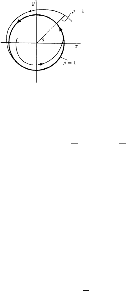
Figure 12.5. The phase plane solution of the differential
equation system (12.12). The asymptotically stable limit
cycle is ρ = 1 and the phase θ = ωt.
plane. If we now change to polar coordinates ρ and θ in the phase plane with
x
1
= ρ cos θ, x
2
= ρ sin θ (12.11)
the system (12.10) becomes
dρ
dt
= ρ(1 −ρ),
dθ
dt
= ω, (12.12)
and the limit cycle is then seen to be ρ = 1. The solution is illustrated in Figure 12.5.
The limit cycle is asymptotically stable since any perturbation from ρ = 1 will die out
by ρ simply winding back onto ρ = 1 and in an anti-clockwise way because dθ/dt > 0.
If the perturbation from the circle is to a point ρ<1 then, from (12.12), ρ increases,
while if the perturbation is to a point ρ>1, ρ decreases as it tends to the orbit ρ = 1.
In this case ρ = 1 is the equivalent of the orbit γ and θ is the phase, which runs from
θ = 0to2π as a circuit is completed.
Returning to the model system (12.9), we take θ to be one of the n variables: its
value is always modulo 2π;thatis,anyvalueθ = θ +2mπ for all integers m. Let us now
consider the remaining n −1 variables, denoted by r, to be perturbations perpendicular
to the limit cycle orbit γ , where we have taken local coordinates such that the actual
orbit γ in an undisturbed state is r = 0. (With the above example in Figure 12.5, this
would be equivalent to changing the variables from (ρ, θ) to (r,θ) where r = 1 − ρ:
the limit cycle orbit γ , ρ = 1, becomes r = 0. Now r = 0 represents a perturbation
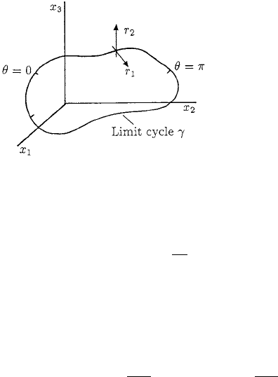
from γ .) Figure 12.6 is an example of this system in the case n = 3.
With the coordinate transformation and parametrisation above, the system (12.9)
can be written as
dr
dt
= f
1
(r,θ), (12.13)
dθ
dt
= ω + f
2
(r,θ), (12.14)
where f
1
(0,θ) = 0 = f
2
(0,θ) and the period of the oscillator is T = 2π/ω.The
functions f
1
and f
2
are periodic in θ with period 2π by virtue of the coordinate system
12.3 Mathematical Model for the Central Pattern Generator 427
Figure 12.6. An example of a phase space for the
system (12.9) for n = 3. Here r has two components r
1
and r
2
with the phase θ being the third component.
we have set up for the limit cycle behaviour of (12.9). If there is no external excitation
the limit cycle is simply
r = 0,
dθ
dt
= ω ⇒ θ(t) = θ(0) +ωt. (12.15)
At each segment there are two coupled oscillators such as we have just described.
They are linked in such a way that if there are no intersegmental influences the out-
puts from the right and left oscillator, denoted by x
R
(t) and x
L
(t) respectively, simply
oscillate 180
◦
out of phase. Each oscillator is of the form (12.9); that is,
dx
R
dt
= f
R
(x
R
, x
L
),
dx
L
dt
= f
L
(x
L
, x
R
). (12.16)
Associated with each of the oscillators is a phase θ
R
and θ
L
and a vector r
R
and r
L
which is the deviation from each oscillator in isolation caused by the intrasegmental
coupling. That is, if there were no coupling the equations in (12.16) would be uncou-
pled, dθ
R
/dt and dθ
L
/dt would each be equal to ω and r
R
, r
L
both equal to zero.
From the experimental observations described in Section 12.2 the pair of segmental
oscillators is 180
◦
out of phase so we assume in the model that
θ
L
(t) = θ
R
(t) +π. (12.17)
Later we include some weak intersegmental coupling so this relationship will only be
a first-order approximation. With such a phase relationship the outputs x
R
and x
L
are
also 180
◦
out of phase which implies
x
L
(t) = x
R
(t + T/2), (12.18)
where T is the common period, which gives a relationship between x
R
and x
L
.This
means that the pair of equations (12.16) can be reduced to a single equation for either
the left or right oscillator. The point is that with this assumed intrasegmental coupling
we end up again with the reduced system (12.13) and (12.14).
With the single oscillator, as the phase θ increases, the output levels of the variables
x(t) vary periodically, typically as illustrated schematically in Figure 12.7. Let us sup-
pose that bursting starts when some output x(t) reaches a threshold value and remains
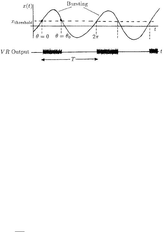
428 12. Oscillator-Generated Wave Phenomena
Figure 12.7. Schematic periodic output x(t) from a single oscillator. When the output level is above a thresh-
old it triggers the VR bursting.
on as long as x(t) is above this threshold value. We can take the value of the phase where
this threshold for x(t) occurs to be θ = 0: we can set the origin of the phase where we
like. Because of the periodic rise and fall of the variable x(t) its value will eventually
pass through the critical threshold value again and the bursting will be shut off. (We
shall see in Chapter 13 and Chapter 1, Volume II that such threshold phenomena occur
in other wave situations.)
Experimentally bursting is observed for only about 0.4 of the period, which in our
scaling is 2π × 0.4. If we let θ
0
be the phase at which bursting ceases, the bursting
based on this then occurs as illustrated in Figure 12.7 for θ + 2mπ,0<θ<θ
0
for all
m = 0, 1, 2,....
Sequence of Coupled Oscillators
We now need to look at the effect on each of the segmental oscillators if they are cou-
pled. So, we now consider the series of segmental oscillators (at each stage there is a
pair but as we showed above the analysis requires a study of only one) which consists
of N equations of the form (12.9), a typical one of which we write as
dx
j
dt
= f
j
(x
j
) +g
j
(x
1
,... ,x
N
, c), j = 1,... ,N, (12.19)
where g represents the coupling effect of the other N −1 oscillators and c is a vector of
coupling parameters. If c = 0 the oscillators are uncoupled; that is, g
j
(x
1
,... ,x
N
, 0) =
0andtheN oscillators then simply have their own periodic limit cycle γ
j
.
The general mathematical problem (12.19) is essentially intractable without some
simplifying assumptions or specialisations. The problem of determining the interaction
properties of coupled oscillators has been widely studied for many years. Hard quantita-
tive results are not trivial to get and most studies have been on a limited number of oscil-
lators, like two, or when the coupling between the oscillators is weak. The mathematics
used covers a wide spectrum, with singular perturbation techniques being among the
most powerful and helpful. We discussed some properties of coupled oscillator systems
in Chapter 9, Sections 9.5 and 9.10. With the above system, some useful and experimen-
tally pertinent results can be obtained if we consider the coupling effects to be weak,
that is, if we assume |c |1and|g ||f |, and then use perturbation methods. The

12.3 Mathematical Model for the Central Pattern Generator 429
implications, or rather assumptions, of this are that the limit cycles γ
j
, j = 1, 2,... ,N
of the isolated oscillators will only be slightly perturbed by the coupling effects (recall
Section 9.5). So, it is still appropriate to use the oscillator equation form (12.13) and
(12.14) involving the phase θ and deviations r
j
from the limit cycle γ
j
, but now we
have to include an extra small coupling term in the equation. (In fact we shall make
even further simplifying assumptions based on what has been observed experimentally,
but it is instructive to proceed a little further with the current line since it is the basis for
a rigourous justification of the assumptions we make later.) The set of N equations we
have to study is then
dr
j
dt
= f
j1
(r
j
,θ
j
) + g
j1
(r
1
,... ,r
N
,θ
1
,... ,θ
N
, c),
dθ
j
dt
= ω
j
+ f
j2
(r
j
,θ
j
) + g
j2
(r
1
,... ,r
N
,θ
1
,... ,θ
N
, c), j = 1, 2,... ,N.
(12.20)
Experimentally it has been observed that the individual oscillators when uncoupled,
by severing and thus isolating them from their neighbours, have different frequencies
ω
j
and hence different periods T
j
= 2π/ω
j
. A crucially important point to keep in
mind is that when the segmental oscillators are coupled they still perform limit cycle
oscillations. So, even when coupled we can still characterise them in terms of their phase
θ
j
. Since fictive swimming is a reflection of phase coupling we need only consider a
phase coupling model for the system (12.19). So, instead of studying the system (12.19)
perturbed about r
j
= 0 we can consider a system of phase coupled equations of the form
dθ
j
dt
= ω
j
+h
j
(θ
1
,... ,θ
N
, c), j = 1,... ,N, (12.21)
where h
j
includes the (weak) coupling effect of all the other oscillators. Equations
(12.21) do not involve the amplitudes of the oscillators. The problem of weak cou-
pling in a population of oscillators has been studied in some depth, for example, by
Neu (1979, 1980), Rand and Holmes (1980), Ermentrout (1981) and in the book by
Guckenheimer and Holmes (1983). Carrying out a perturbation of (12.19) about r
j
= 0
eventually results in a phase coupled system of equations (12.21) (see Chapter 9). So,
there is a mathematical, as well as biological, justification for considering the simpler
model (12.21).
Since we assume small perturbations from the individual limit cycle oscillators to
come from the coupling, it is reasonable to consider a linear coupling model where the
effect of the jth oscillator on the ith one is simply proportional to x
j
. In this situation
the coupled oscillator system is of the form (12.9) perturbed by linear terms; namely,
dx
i
dt
= f
i
(x
i
) +
N
j=1
j=i
A
ij
x
j
, (12.22)
where A
ij
are matrices of the coupling coefficients.
430 12. Oscillator-Generated Wave Phenomena
Equations (12.22) include both the phases and amplitudes. We argued above that
we need only consider a phase coupled model so even (12.22) is more complicated than
we need consider. It was shown in Chapter 9, Section 9.9 (see also Neu 1979, 1980 and
Rand and Holmes 1980) that, in the case of weak coupling, (12.22) leads to a phase
coupled system of differential equations of the form
dθ
i
dt
= ω
i
+
N
j=1
a
ij
h(θ
j
−θ
i
), i = 1,... ,N, (12.23)
where h is a periodic function of its argument. We can argue heuristically, however,
to justify the model system (12.23). Since we suggested that we need only consider a
phase model, a linear coupling would reasonably involve a coupling term which was a
function of the phase differences of the oscillator and all the others in the system. The
periodic nature of the function h is suggested by the fact that we would also reasonably
expect the phase difference between any two oscillators to be periodic. There is, as well,
experimental evidence to support such a conjecture from Buchanan and Cohen (1982),
who found that the slowly varying intrasegmental potentials of the motoneurons are
quasi-sinusoidal. As the specific model to study therefore we take the simple periodic
function h(φ) = sin φ in (12.23). For a discussion of a more general h in the case of
coupled oscillators, see Kopell (1988).
The phase coupled model we analyse in detail is the set of N phase equations
dθ
i
dt
= ω
i
+
N
j=1
j=i
a
ij
sin(θ
j
−θ
i
), i = 1,... ,N. (12.24)
The a
ij
s are a measure of the effect of the jth oscillator on the ith one with the effect
being excitatory, meaning θ
j
tends to pull θ
i
towards its value if a
ij
is positive, while it
is inhibitory if a
ij
is negative. In the inhibitory case θ
j
tends to increase the difference
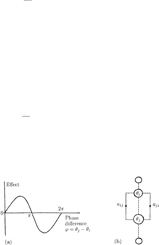
Figure 12.8. (a) Measure of the effect on the ith oscillator of the jth oscillator for a sinusoidal form for the
interaction function h(φ) of the phase difference. (b) Schematic representation of the coupling of the ith and
jth oscillators according to (12.24).

12.4 Analysis of the Phase Coupled Model System 431
between it and θ
i
. With the specific interaction function sin φ we choose for h in (12.23)
the maximum excitatory effect of the jth oscillator on the ith one is when they are π/2
out of phase; the maximum inhibitory effect is when they are −π/2 out of phase with
no effect when they are in phase. Figure 12.8 schematically illustrates the model and
the sinusoidal coupling effect.
We wish to retain in our model the periodic character of the oscillators when they
are coupled. More particularly we want dθ
i
/dt always to be a positive and monotonic
increasing function of t, so that movement on the limit cycle γ
i
is always in one di-
rection, or in other words so that the output has a regular up and down character as in
Figure 12.8(a). We assume therefore that the magnitudes of ω
i
and a
ij
are such that
the phase θ
i
(t) behaves in this way. We now wish to analyse the model system (12.24)
and see whether or not it is a reasonable model when the solutions are compared with
experimental results.
12.4 Analysis of the Phase Coupled Model System
We have to decide what kind of coupling we wish to include in the model system
(12.24). Here we analyse the simplest, namely, when each oscillator is only coupled
to its nearest neighbours. In this case (12.24) becomes the coupled system of N equa-
tions
dθ
1
dt
= ω
1
+a
12
sin(θ
2
−θ
1
)
dθ
2
dt
= ω
2
+a
21
sin(θ
1
−θ
2
) + a
23
sin(θ
3
−θ
2
)
.
.
.
dθ
j
dt
= ω
j
+a
j, j−1
sin(θ
j−1
−θ
j
) +a
j, j+1
sin(θ
j+1
−θ
j
)
.
.
.
dθ
N
dt
= ω
N
+a
N,N−1
sin(θ
N−1
−θ
N
).
(12.25)
The form of the right-hand sides suggests that we introduce
φ
j
= θ
j
−θ
j+1
,
j
= ω
j
−ω
j+1
(12.26)
and rewrite the system (12.25) in terms of the φ’s, the phase differences, and the ’s,
the frequency differences, by subtracting the θ-equations pairwise to get the N − 1
equations

432 12. Oscillator-Generated Wave Phenomena
dφ
1
dt
=
1
−(a
12
+a
21
) sin φ
1
+a
23
sin φ
2
dφ
2
dt
=
2
+a
21
sin φ
1
−(a
23
+a
32
) sin φ
2
+a
34
sin φ
3
.
.
.
dφ
j
dt
=
j
+a
j, j−1
sin φ
j−1
−(a
j, j+1
+a
j+1, j
) sin φ
j
+a
j+1, j+2
sin φ
j+1
.
.
.
dφ
N−1
dt
=
N−1
+a
N−1,N −2
sin φ
N−2
−(a
N−1,N
+a
N,N−1
) sin φ
N−1
.
(12.27)
Since we are looking for some regular periodic pattern which we associate with fictive
swimming, we can make some assumptions about the coupling coefficients a
ij
.(We
are also trying to get the simplest reasonable model to mimic the experimental phe-
nomenon.) Let us assume that all the upward (in number, that is—in our model this is
in the head-to-tail direction) coupling coefficients a
j, j+1
= a
u
and all the downwards
coefficients a
j, j−1
= a
d
. The system (12.27) in vector form is then
dφ
dt
= + BS, (12.28)
where the vectors
φ =
φ
1
.
.
.
φ
N−1
, S =
sin φ
1
.
.
.
sin φ
N−1
,=
1
.
.
.
N−1
(12.29)
and B is the (N − 1) ×(N −1) matrix
B =
−(a
d
+a
u
) a
u
··
a
d
−(a
d
+a
u
) a
u
·
· ···
· ···
··a
d
−(a
d
+a
u
)
. (12.30)
For the application of the model to the fictive swimming of the lamprey, we are
interested in phase locked solutions of (12.28). That is, the coupling must be such that all
the oscillators have the same period. This is the same as saying that the phase differences
φ
j
between the oscillators is always constant for all j = 1, 2,... ,N − 1. This in turn
means that dφ
j
/dt = 0 and so we are looking for equilibrium solutions of (12.28), that
is, the solutions of
0 = +BS ⇒ S =−B
−1
. (12.31)
Since S involves only sin φ
j
, j = 1, 2,... ,N−1, solutions exist only if all the elements
of B
−1
lie between ±1.
12.4 Analysis of the Phase Coupled Model System 433
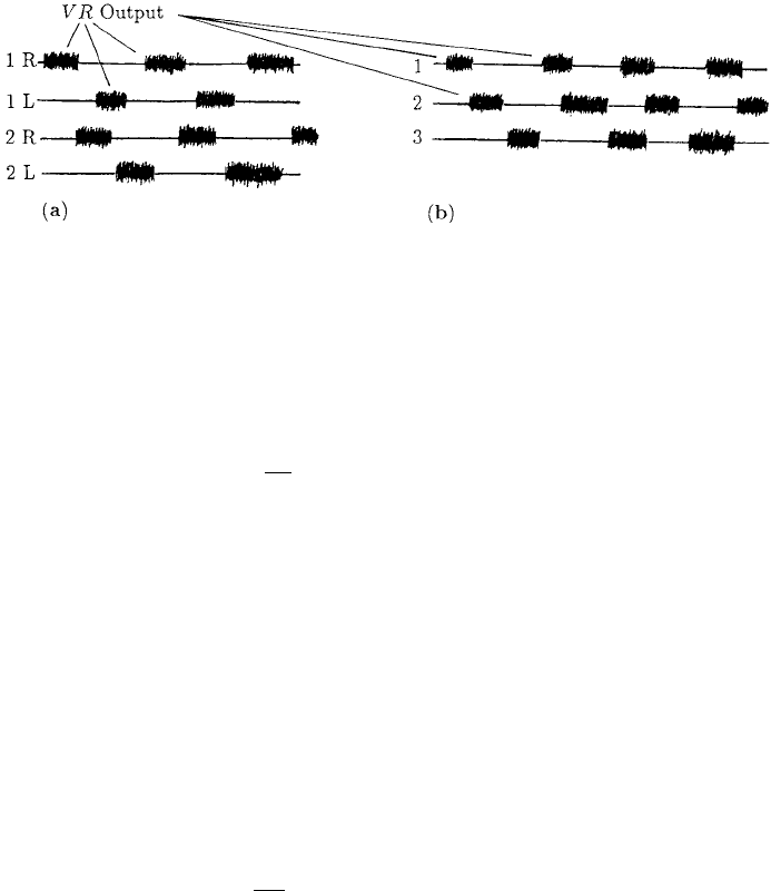
Figure 12.9. (a) Ventral root output from a phase locked 2-oscillator model. (b) Ventral root output from a
phase locked solution of a 3-oscillator system: note that the phase difference between the 1st and 2nd root is
not necessarily the same as between the 2nd and 3rd.
Two-Oscillator System
Here we have only a single equation for the phase difference φ = θ
1
−θ
2
; namely,
dφ
dt
= −(a
d
+a
u
) sin φ. (12.32)
This has phase locked solutions, where dφ/dt = 0, if and only if
| |≤|a
d
+a
u
|. (12.33)
If we denote the solutions by φ
S
then if
| |=|a
d
+a
u
| then φ
S
= π/2or3π/2,
| | < |a
d
+a
u
| then |φ
S
| <π/2orπ/2 < |φ
S
|≤π.
(12.34)
We can determine the stability of these steady state solutions by linearising about them
in the usual way (as in Chapter 1, Section 1.1). If we denote perturbations about φ
S
by
ψ, the linear stability equation from (12.32) is
dψ
dt
≈−[(a
d
+a
u
) cos φ
S
]ψ.
The first two possible solutions in (12.34) are neutrally stable, because cos φ
S
= 0,
while one of the second set is stable and the other unstable. So, as the coupling strength
|a
d
+a
u
| decreases relative to the frequency difference | |, | |/|a
d
+a
u
| increases
and the stable steady state, as well as the unstable one, tends to the neutrally stable
one as |a
d
+ a
u
|→| | after which no solution exists. Thus as the coupling strength
|a
d
+a
u
| becomes weaker relative to the detuning | |=ω
1
−ω
2
a bifurcation takes
place where the stable phase locked solution ceases to exist. The stable steady state
when it exists, is the phase locked solution we are interested in. From the discussion
above in Section 12.2, a model with two oscillators has two pairs of ventral roots and,
with the threshold bursting implied by Figure 12.7 and phase difference at each VR pair,
the bursting output is as illustrated in Figure 12.9(a).

434 12. Oscillator-Generated Wave Phenomena
Three-Oscillator System
The steady states for this system are, from (12.31),
sin φ
1
sin φ
2
=
1
a
2
d
+a
d
a
u
+a
2
u
a
d
+a
u
a
u
a
d
a
d
+a
u
1
2
. (12.35)
For algebraic simplicity let us take the coupling coefficients a
d
= a
u
= a,inwhich
case the last equation gives
sin φ
1
= (2
1
+
2
)/3a, sin φ
2
= (
1
+2
2
)/3a. (12.36)
Thus a phase locked solution (φ
1
,φ
2
) exists if and only if
max{|2
1
+
2
|/3a, |
1
+2
2
|/3a} < 1. (12.37)
In this 3-oscillator case the phase differences φ
1
and φ
2
are unequal in general, and a
typical VR output from it is schematically illustrated in Figure 12.9(b).
As the number of oscillators increases the algebraic complexity quickly gets out of
hand but it is clear how to set up the algebraic problem to be solved, that is, how to get
the set of conditions that must hold between the coupling coefficients and the detuning
parameters for a phase locked solution to exist.
Constant Phase Lag System of N-Oscillators
To keep the generality in a multi-oscillator model such as we did with the last two sys-
tems is perhaps unnecessarily cumbersome. What we wish to show is that such coupled
oscillators can give a stable phase locked system, such as required by a central pattern
generator to produce the required VR output necessary for fictive swimming. So, here
we consider a system where there is a constant phase lag between neighbouring seg-
ments; that is, we assume that the phase difference φ
j
= θ
j
− θ
j+1
= δ, a positive
constant. This situation is of particular relevance to the experimental facts related to
Figure 12.3. Such a line of oscillators is characteristic of a uniform travelling wave.
Although the analysis here can be done with any periodic h in (12.23) (see Exercise 2),
we continue to use the example h(φ) = sin φ for consistency. If we set = sin δ>0
the system of equations for the steady states becomes, from (12.31) with (12.29) and
(12.30),
1
+[−(a
d
+a
u
) + a
u
] = 0 ⇒
1
= a
d
.
.
.
j
+[a
d
−(a
d
+a
u
) + a
u
] = 0 ⇒
j
= 0, j = 2,... ,N − 2
.
.
.
N−1
+[a
d
−(a
d
+a
u
)] = 0 ⇒
N−1
= a
u
.
(12.38)

12.4 Analysis of the Phase Coupled Model System 435
In terms of the original frequencies, since
j
= ω
j
−ω
j+1
,thisgives
ω
j
= ω for all j = 2,... ,N −1
ω
1
= ω +a
d
sin δ>ω
ω
N
= ω −a
u
sin δ<ω.
(12.39)
What this solution means is that all the oscillators except the first, the rostral or head
oscillator, and the last, the caudal or tail oscillator, have the natural frequency of each
segmental oscillator in isolation. The head oscillator is tuned up, that is, to a higher
frequency, while the tail one is tuned down. This assumes that the coupling coefficients
a
d
and a
u
in (12.39) are positive; that is, the coupling is excitatory. The resulting wave
which results from this is one which travels from head to tail. Another solution to this
constant phase lag problem is when the head oscillator is tuned down and the tail one
tuned up. This results in the wave propagating from tail to head; that is, the lamprey
swims backwards, which in fact it can do.
We finally have to consider the stability of this constant phase lag solution. We do
this in the usual way by linearising about φ
j
= δ by writing
φ
j
= δ +ψ
j
, j = 1,... ,N, (12.40)
where ||ψ || 1. Substituting this into the time-dependent equation (12.28) and lin-
earising gives
dψ
dt
= Bψ cos δ, (12.41)
where the matrix B is given by (12.30), depends only on the coupling coefficients a
d
and a
u
and is a tridiagonal (N − 1) × (N − 1) matrix. If we now look for solutions of
(12.41) in the form
ψ(t) = e
λt
ψ
0
(12.42)
the eigenvalues λ are solutions of
|B cos δ −λI |=0, (12.43)
where I is the unit (N − 1) × (N − 1) matrix. From experimental observation phase
lags between segments are quite small and 0 < cos δ<1. Under these circumstances it
can be shown, for example, by using the Routh–Hurwitz conditions on the polynomial
in λ,thatReλ<0. So from (12.42) ψ(t) → 0ast →∞which means that the phase
locked constant phase difference solution above is stable to linear perturbations.
There are of course two solutions for the phase difference equation sin φ
j
= sin δ,
which gives 2
N−1
− 2 other phase locked solutions. However, it can be shown, from a
study of the eigenvalue matrix, that all of them are linearly unstable; that is, there exists
at least one eigenvalue λ in (12.42) with Re λ>0. We conclude therefore, that the
solution (12.39) is the relevant one when there is a constant phase difference between
