Mitchell Т. Machine learning

Подождите немного. Документ загружается.

CHAPTER

REINFORCEMENT

LEARNING

379

during which each

is visited, the largest error in the table will be at most

yAo.

After

such intervals, the error will be at most

ykAo.

Since each state is visited

infinitely often, the number of such intervals is infinite, and

oo.

This proves the theorem.

13.3.5 Experimentation Strategies

Notice the algorithm of Table 13.1 does not specify how actions are chosen by the

agent. One obvious strategy would be for the agent in state

to select the action

that maximizes

~(s,

a),

thereby exploiting its current approximation

However,

with this strategy the agent runs the risk that it will overcommit to actions that

are found during early training to have high

values, while failing to explore

other actions that have even higher values. In fact, the convergence theorem above

requires that each state-action transition occur infinitely often. This will clearly

not occur if the agent always selects actions that maximize its current

&(s,

a).

For

this reason, it is common in

learning to use a probabilistic approach to selecting

actions. Actions with higher

values are assigned higher probabilities, but every

action is assigned a nonzero probability. One way to assign such probabilities is

where

P(ai 1s)

is the probability of selecting action

ai,

given that the agent is in

state

and where

is a constant that determines how strongly the selection

favors actions with high

values. Larger values of

will assign higher proba-

bilities to actions with above average

causing the agent to

exploit

what it has

learned and seek actions it believes will maximize its reward.

contrast, small

values of

will allow higher probabilities for other actions, leading the agent

explore

actions that do not currently have high

values. In some cases,

varied with the number of iterations so that the agent favors exploration during

early stages of learning, then gradually shifts toward a strategy of exploitation.

13.3.6 Updating Sequence

One important implication of the above convergence theorem is that

learning

need not train on optimal action sequences in order to converge to the optimal

policy. In fact, it can learn the

function (and hence the optimal policy) while

training from actions chosen completely at random at each step, as long as the

resulting training sequence visits every state-action transition infinitely often. This

fact suggests changing the sequence of training example transitions in order to

improve training efficiency without endangering final convergence. To illustrate,

consider again learning in an

MDP

with a single absorbing goal state, such as the

one in Figure 13.1. Assume

before that we train the agent with a sequence of

episodes. For each episode, the agent is placed in a random initial state and is

allowed to perform actions and to update its

table until it reaches the absorbing

goal state.

new training episode is then begun by removing the agent from the

goal state and placing it at a new random initial state. As noted earlier, if we

begin with all

values initialized to zero, then after the first full episode only

one entry in the agent's

table will have been changed: the entry corresponding

to the final transition into the goal state. Note that if the agent happens to follow

the same sequence of actions from the same random initial state in its second full

episode, then a second table entry would be made nonzero, and so on. If we run

repeated identical episodes in this fashion, the frontier of nonzero

values will

creep backward from the goal state at the rate of one new state-action transition

per episode. Now consider training on these same state-action transitions, but in

reverse chronological order for each episode. That is, we apply the same update

rule from Equation (13.7) for each transition considered, but perform these updates

in reverse order. In this case, after the first full episode the agent will have updated

its

estimate for every transition along the path it took to the goal. This training

process will clearly converge in fewer iterations, although it requires that the agent

use more memory to store the entire episode before beginning the training for that

episode.

A second strategy for improving the rate of convergence is to store past

state-action transitions, along with the immediate reward that was received, and

retrain on them periodically. Although at first it might seem a waste of effort to

retrain on the same transition, recall that the updated

~(s,

value is determined

by the values

~(s',

of the successor state

6(s,

a).

Therefore, if subsequent

training changes one of the

~(s',

values, then retraining on the transition

(s,

may result in an altered value for

~(s,

a).

In general, the degree to which we wish

to replay old transitions versus obtain new ones from the environment depends

on the relative costs of these two operations in the specific problem domain. For

example, in a robot domain with navigation actions that might take several seconds

to perform, the delay in collecting a new state-action transition from the external

world might be several orders of magnitude more costly than internally replaying

a previously observed transition. This difference can be very significant given that

learning can often require thousands of training iterations to converge.

Note throughout the above discussion we have kept our assumption that the

agent does not know the state-transition function

6(s,

used by the environment

to create the successor state

S(s,

a),

or the function

r(s,

used to generate

rewards. If it does know these two functions, then many more efficient methods

are possible. For example, if performing external actions is expensive the agent

may simply ignore the environment and instead simulate it internally, efficiently

generating simulated actions and assigning the appropriate simulated rewards.

Sutton (1991) describes the

DYNA

architecture that performs a number of simulated

actions after each step executed in the external world. Moore and Atkeson (1993)

describe an approach called

prioritized sweeping

that selects promising states to

update next, focusing on predecessor states when the current state is found to

have a large update. Peng and Williams (1994) describe a similar approach. A

large number of efficient algorithms from the field of dynamic programming can

be applied when the functions

and

are known. Kaelbling et al. (1996) survey

a number of these.

CHAPTER

REINFORCEMENT LEARNING

381

13.4

NONDETERMINISTIC REWARDS AND ACTIONS

Above we considered

learning in deterministic environments. Here we consider

the nondeterministic case, in which the reward function

r(s,

and action transi-

tion function

6(s,

may have probabilistic outcomes. For example, in Tesaur~'~

(1995) backgammon playing program, action outcomes are inherently probabilis-

tic because each move involves a roll of the dice. Similarly, in robot problems

with noisy sensors and effectors it is often appropriate to model actions and re-

wards as nondeterministic. In such cases, the functions

6(s,

and

r(s,

can be

viewed as first producing a probability distribution over outcomes based on

and

and then drawing an outcome at random according to this distribution. When

these probability distributions depend solely on

and

(e.g., they do not depend

on previous states or actions), then we call the system a nondeterministic Markov

decision process.

In this section we extend the

learning algorithm for the deterministic

case to handle

nondeterministic

MDPs. To accomplish this, we retrace the line

of argument that led to the algorithm for the deterministic case, revising it where

needed.

In the nondeterministic case we must first restate the objective of the learner

to take into account the fact that outcomes of actions are no longer

deterministic.

The obvious generalization is to redefine the value

of a policy

to be the

ex-

pected value

(over these nondeterministic outcomes) of the discounted cumulative

reward received by applying this policy

where, as before, the sequence of rewards

r,+i

is generated by following policy

beginning at state

Note this is a generalization of Equation (13.1), which

covered the deterministic case.

As before, we define the optimal policy

to be the policy

that maxi-

mizes

V"(s)

for all states

Next we generalize our earlier definition of

from

Equation (13.4), again by taking its expected value.

where

P(slls,

is the probability that taking action

in state

will produce the

next state

s'.

Note we have used

P(slls,

here to rewrite the expected value of

V*(6(s,

a))

in terms of the probabilities associated with the possible outcomes of

the probabilistic

As before we can re-express

recursively

Q(s,

E[r(s,

a)]

P(sfls,

Q(sl,

a')

(13.9)

which is the generalization of the earlier Equation

(13.6).

To summarize, we have

simply redefined

Q(s, a)

in the nondeterministic case to be the expected value of

its previously defined quantity for the deterministic case.

Now that we have generalized the definition of

to accommodate the non-

deterministic environment functions

and

a new training rule is needed. Our

earlier training rule derived for the deterministic case (Equation

13.7)

fails to con-

verge in this nondeterministic setting. Consider, for example, a nondeterministic

reward function

r(s, a)

that produces different rewards each time the transition

(s, a}

is repeated. In this case, the training rule will repeatedly alter the values of

Q(S, a),

even if we initialize the

table values to the correct

function. In brief,

this training rule does not converge. This difficulty can be overcome by modifying

the training rule so that it takes a decaying weighted average of the current

value and the revised estimate. Writing

to denote the agent's estimate on the

nth iteration of the algorithm, the following revised training rule is sufficient to

assure convergence of

Q~(s, a)

un)Qn-l(s, a)

a,[r

max

Q,-~(S', a')]

(13.10)

where

visits, (s, a)

where

and

here are the state and action updated during the nth iteration, and

where

visits,(s, a)

is the total number of times this state-action pair has been

visited up to and including the nth iteration.

The key idea in this revised rule is that revisions to

are made more

gradually than in the deterministic case. Notice if we were to set

Equation

(13.10)

we would have exactly the training rule for the deterministic case.

With smaller values of

this term is now averaged in with the current

~(s, a)

produce the new updated value. Notice that the value of

in Equation

(13.11)

decreases as n increases, so that updates become smaller as training progresses.

By reducing

at an appropriate rate during training, we can achieve convergence

to the correct

function. The choice of

given above is one of many that

satisfy the conditions for convergence, according to the following theorem due to

Watkins and Dayan

(1992).

Theorem

13.2.

Convergence of

learning for nondeterministic Markov de-

cision processes.

Consider a

learning agent in a nondeterministic

MDP

with

bounded rewards

(Vs, a)lr(s, a)l

The

learning agent uses the training rule of

Equation

(13.10),

initializes its table

~(s, a)

to arbitrary finite values, and uses a

discount factor

such that

Let

n(i, s, a)

be the iteration corresponding

to the

ith

time that action

is applied to state

If each state-action pair is visited

infinitely often,

a,,

and

then for all

and

a, &,(s, a)

Q(s, a)

00,

with probability

While

learning and related reinforcement learning algorithms can be

proven to converge under certain conditions, in practice systems that use

learn-

ing often require many thousands of training iterations to converge. For exam-

ple, Tesauro's

TD-GAMMON

discussed earlier trained for

1.5

million backgammon

games, each of which contained tens of state-action transitions.

13.5

TEMPORAL DIFFERENCE LEARNING

The

learning algorithm learns by iteratively reducing the discrepancy between

value estimates for adjacent state:,.

this sense,

learning is a special case

of a general class of

temporal diflerence

algorithms that learn by reducing dis-

crepancies between estimates made by the agent at different times. Whereas the

training rule of Equation (13.10) reduces the difference between the estimated

values of a state and its immediate successor, we could just as well design an algo-

rithm that reduces discrepancies between this state and more distant descendants

or ancestors.

To explore this issue further, recall that our

learning training rule calcu-

lates a training value for

&(st, a,)

in terms of the values for

&(s,+l, at+l)

where

s,+l

is the result of applying action

to the state

st.

Let

Q(')(s,, a,)

denote the

training value calculated by this one-step lookahead

One alternative way to compute a training value for

Q(s,, a,)

is to base it on the

observed rewards for two steps

st,

a,)

yr,+l

max

Q(s~+~, a)

or, in general, for

steps

Q(~)(s,,~,)

yr,+l

,-.

y(n-l)rt+n-l

ynmax&(s,+,,a)

Sutton (1988) introduces a general method for blending these alternative

training estimates, called

TD(h).

The idea is to use a constant 0

1 to

combine the estimates obtained from various lookahead distances in the following

fashion

An equivalent recursive definition for

Note if we choose

0 we have our original training estimate

Q('),

which

considers only one-step discrepancies in the

estimates. As

is increased, the al-

gorithm places increasing emphasis on discrepancies based on more distant looka-

heads. At the extreme value

1, only the observed

r,+i

values are considered,

with no contribution from the current

estimate. Note when

Q, the training

values given by Qh will be identical for all values of h such that

The motivation for the TD(h) method is that in some settings training will

be more efficient if more distant lookaheads are considered. For example, when

the agent follows an optimal policy for choosing actions, then

with h

1 will

provide a perfect estimate for the true Q value, regardless of any inaccuracies in

the other hand, if action sequences are chosen suboptimally, then the

r,+i

observed far into the future can be misleading.

Peng and Williams (1994) provide a further discussion and experimental

results showing the superior performance of Qqn one problem domain. Dayan

(1992) shows that under certain assumptions a similar TD(h) approach applied

to learning the

function converges correctly for any h such that

Tesauro (1995) uses a TD(h) approach in his TD-GAMMON program for playing

backgammon.

13.6

GENERALIZING FROM EXAMPLES

Perhaps the most constraining assumption in our treatment of Q learning up to

this point is that the target function is represented as an explicit lookup table,

with a distinct table entry for every distinct input value (i.e., state-action pair).

Thus, the algorithms we discussed perform a kind of rote learning and make

no attempt to estimate the Q value for unseen state-action pairs by generalizing

from those that have been seen. This rote learning assumption is reflected in the

convergence proof, which proves convergence only if every possible state-action

pair is visited (infinitely often!). This is clearly an unrealistic assumption in large

or infinite spaces, or when the cost of executing actions is high. As a result,

more practical systems often combine function approximation methods discussed

in other chapters with the Q learning training rules described here.

It is easy to incorporate function approximation algorithms such as

BACK-

PROPAGATION

into the Q learning algorithm, by substituting a neural network for

the lookup table and using each ~(s, a) update as a training example. For example,

we could encode the state

s and action a as network inputs and train the network

to output the target values of

given by the training rules of Equations (13.7)

and (13.10).

alternative that has sometimes been found to be more successful

in practice is to train a separate network for each action, using the state as input

and

as output. Another common alternative -is to train one network with the

state as input, but with one

output for each action. Recall that in Chapter

discussed approximating an evaluation function over checkerboard states using a

linear function and the

LMS

algorithm.

In practice, a number of successful reinforcement learning systems have been

developed by incorporating such function approximation algorithms in place of the

lookup table. Tesauro's successful TD-GAMMON program for playing backgammon

used a neural network and the

BACKPROPAGATION algorithm together with a TD(A)

training rule. Zhang and Dietterich (1996) use a similar combination of BACKPROP-

AGATION

and TD(h) for job-shop scheduling tasks. Crites and Barto (1996) describe

a neural network reinforcement learning approach for an elevator scheduling task.

Thrun (1996) reports a neural network based approach to

learning to learn basic

control procedures for a mobile robot with sonar and camera sensors. Mahadevan

and Connell (1991) describe a

learning approach based on clustering states,

applied to a simple mobile robot control problem.

Despite the success of these systems, for other tasks reinforcement learning

fails to converge once a generalizing function approximator is introduced. Ex-

amples of such problematic tasks are given by Boyan and Moore (1995), Baird

(1995), and Gordon (1995). Note the convergence theorems discussed earlier in

this chapter apply only when

is represented by an explicit table. To see the

difficulty, consider using a neural network rather than an explicit table to repre-

sent

Note if the learner updates the network to better fit the training

value

for a particular transition (si, ai), the altered network weights may also change

the

estimates for arbitrary other transitions. Because these weight changes may

increase the error in

estimates for these other transitions, the argument prov-

ing the original theorem no longer holds. Theoretical analyses of reinforcement

learning with generalizing function approximators are given by Gordon (1995)

and Tsitsiklis (1994). Baird (1995) proposes gradient-based methods that circum-

vent this difficulty by directly minimizing the sum of squared discrepancies in

estimates between adjacent states (also called

Bellman residual errors).

13.7

RELATIONSHIP TO DYNAMIC PROGRAMMING

Reinforcement learning methods such as

learning are closely related to a long

line of research on dynamic programming approaches to solving Markov decision

processes. This earlier work has typically assumed that the agent possesses perfect

knowledge of the functions

S(s,

and r(s,

that define the agent's environment.

Therefore, it has primarily addressed the question of how to compute the optimal

policy using the least computational effort, assuming the environment could be

perfectly simulated and no direct interaction was required. The novel aspect of

learning is that it assumes the agent does

not

have knowledge of

S(s,

and

r(s,

a),

and that instead of moving about in an internal mental model of the state

space, it must move about the real world and observe the consequences.

this

latter case our primary concern is usually the number of real-world actions that the

agent must perform to converge to an acceptable policy, rather than the number of

computational cycles it must expend. The reason is that in many practical domains

such as manufacturing problems, the costs in time and in dollars of performing

actions in the external world dominate the computational costs. Systems that learn

by moving about the real environment and observing the results are typically called

online

systems, whereas those that learn solely by simulating actions within

internal model are called

ofline

systems.

The close correspondence between these earlier approaches and the rein-

forcement learning problems discussed here is apparent by considering Bellman's

equation, which forms the foundation for many dynamic programming approaches

to solving MDPs. Bellman's equation is

Note the very close relationship between Bellman's equation and our earlier def-

inition of an optimal policy in Equation (13.2). Bellman (1957) showed that the

optimal policy

satisfies the above equation and that any policy

satisfying

this equation is an optimal policy. Early work on dynamic programming includes

the Bellman-Ford shortest path algorithm (Bellman 1958; Ford and Fulkerson

1962), which learns paths through a graph by repeatedly updating the estimated

distance to the goal for each graph node, based on the distances for its neigh-

bors. In this algorithm the assumption that graph edges and the goal node are

known is equivalent to our assumption that

6(s,

and

r(s,

are known. Barto

et al. (1995) discuss the close relationship between reinforcement learning and

dynamic programming.

13.8

SUMMARY AND FURTHER READING

The key points discussed in this chapter include:

Reinforcement learning addresses the problem of learning control strategies

for autonomous agents. It assumes that training information is available in

the form of a real-valued reward signal given for each state-action transition.

The goal of the agent is to learn an action policy that maximizes the total

reward it will receive from any starting state.

The reinforcement learning algorithms addressed in this chapter fit a problem

setting known as a Markov decision process. In Markov decision processes,

the outcome of applying any action to any state depends only on this ac-

tion and state (and not on preceding

actions:or states). Markov decision

processes cover a wide range of problems including many robot control,

factory automation, and scheduling problems.

learning is one form of reinforcement learning in which the agent learns

an evaluation function over states and actions. In particular, the evaluation

function

Q(s,

is defined as the maximum expected, discounted, cumulative

reward the agent can achieve by applying action

to state

The

learning

algorithm has the advantage that it can-be employed even when the learner

has no prior knowledge of how its actions affect its environment.

learning can be proven to converge to the correct

function under cer-

tain assumptions, when the learner's hypothesis

~(s,

is represented by a

lookup table with a distinct entry for each

(s,

pair. It can be shown to

converge in both deterministic and nondeterministic MDPs. In practice,

learning can require many thousands of training iterations to converge in

even modest-sized problems.

learning is a member of a more general class of algorithms, called tem-

poral difference algorithms.

general, temporal difference algorithms learn

CHAFER

REINFORCEMENT

LEARNING

387

by iteratively reducing the discrepancies between the estimates produced by

the agent at different times.

Reinforcement learning is closely related to dynamic programming ap-

proaches to Markov decision processes. The key difference is that histori-

cally these dynamic programming approaches have assumed that the agent

possesses knowledge of the state transition function

6(s, a) and reward func-

tion

a). In contrast, reinforcement learning algorithms such as

learning

typically assume the learner lacks such knowledge.

The common theme that underlies much of the work on reinforcement learn-

ing is to iteratively reduce the discrepancy between evaluations of successive

states. Some of the earliest work on such methods is due to Samuel (1959). His

checkers learning program attempted to learn an evaluation function for checkers

by using evaluations of later states to generate training values for earlier states.

Around the same time, the Bellman-Ford, single-destination, shortest-path algo-

rithm was developed (Bellman 1958; Ford and Fulkerson 1962), which propagated

distance-to-goal values from nodes to their neighbors. Research on optimal control

led to the solution of Markov decision processes using similar methods

(Bellman

1961; Blackwell 1965). Holland's (1986) bucket brigade method for learning clas-

sifier systems used a similar method for propagating credit in the face of delayed

rewards. Barto et

al.

(1983) discussed an approach to temporal credit assignment

that led to Sutton's paper (1988) defining the TD(k) method and proving its con-

vergence for k

Dayan (1992) extended this result to arbitrary values of k.

Watkins (1989) introduced

learning to acquire optimal policies when the re-

ward and action transition functions are unknown. Convergence proofs are known

for several variations on these methods. In addition to the convergence proofs

presented in this chapter see, for example, (Baird 1995; Bertsekas 1987; Tsitsiklis

1994, Singh and Sutton 1996).

Reinforcement learning remains an active research area.

McCallum (1995)

and Littman (1996), for example, discuss the extension of reinforcement learning

to settings with hidden state variables that violate the Markov assumption. Much

current research seeks to scale up these methods to larger, more practical prob-

lems. For example, Maclin and Shavlik (1996) describe an approach in which a

reinforcement learning agent can accept imperfect advice from a trainer, based on

an extension to the

KBANN

algorithm (Chapter 12). Lin (1992) examines the role

of teaching by providing suggested action sequences. Methods for scaling Up by

employing a hierarchy of actions are suggested by Singh (1993) and Lin (1993).

Dietterich and

Flann (1995) explore the integration of explanation-based methods

with reinforcement learning, and Mitchell and

Thrun (1993) describe the appli-

cation of the

EBNN

algorithm (Chapter 12) to

learning. Ring (1994) explores

continual learning

the agent over multiple tasks.

Recent surveys of reinforcement learning are given by Kaelbling et al.

(1996);

Barto

(1992);

Barto et al. (1995); Dean et al. (1993).

EXERCISES

13.1.

Give a second optimal policy for the problem illustrated in Figure

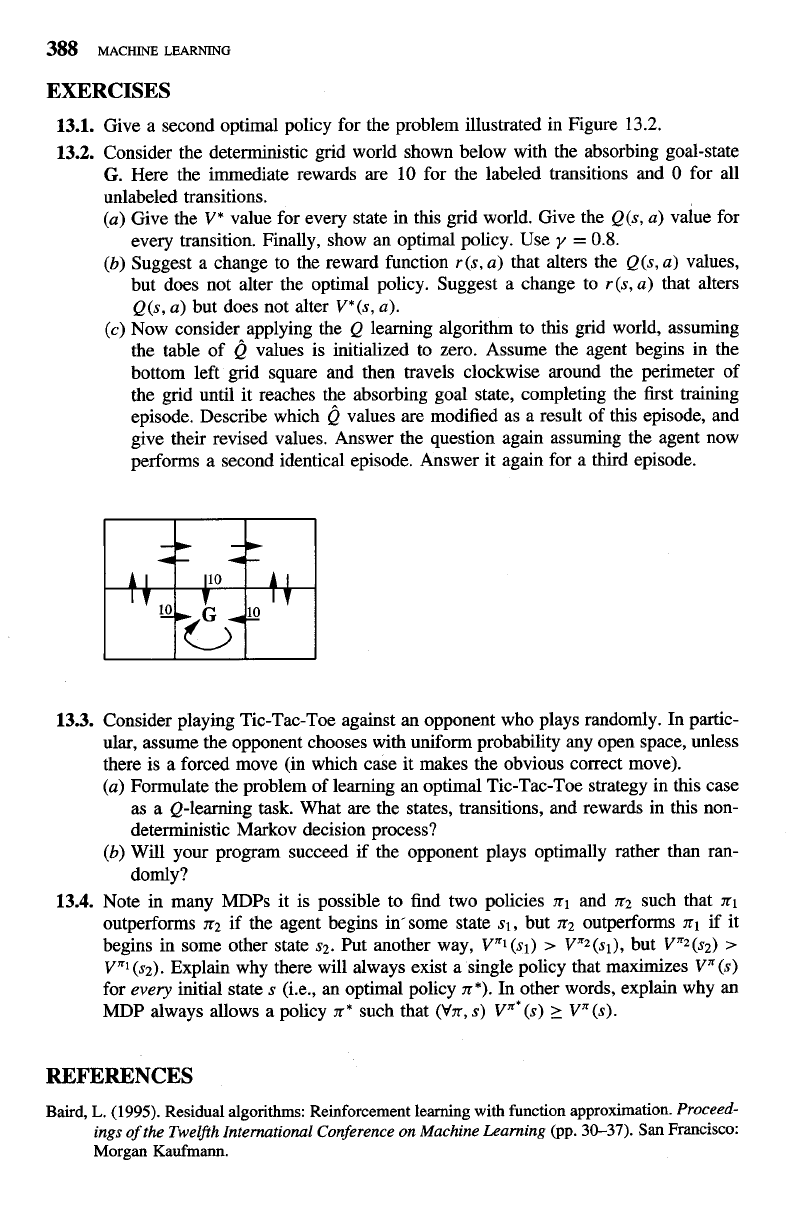
13.2.

Consider the deterministic grid world shown below with the absorbing goal-state

Here the immediate rewards are

for the labeled transitions and

for all

unlabeled transitions.

(a) Give the V* value for every state in this grid world. Give the

Q(s, a) value for

every transition. Finally, show an optimal policy. Use

0.8.

(b)

Suggest a change to the reward function r(s, a) that alters the Q(s, a) values,

but does not alter the optimal policy. Suggest a change to r(s, a) that alters

Q(s, a) but does not alter V*(s, a).

the table of

values is initialized to zero. Assume the agent begins in the

bottom left grid square and then travels clockwise around the perimeter of

the grid until it reaches the absorbing goal state, completing the first training

episode. Describe which

values are modified as a result of this episode, and

give their revised values. Answer the question again assuming the agent now

performs a second identical episode. Answer it again for a third episode.

13.3.

Consider playing Tic-Tac-Toe against an opponent who plays randomly. In partic-

ular, assume the opponent chooses with uniform probability any open space, unless

there is a forced move (in which case it makes the obvious correct move).

(a) Formulate the problem of learning an optimal Tic-Tac-Toe strategy in this case

as a Q-learning task. What are the states, transitions, and rewards in this non-

deterministic Markov decision process?

(b)

Will your program succeed if the opponent plays optimally rather than ran-

domly?

13.4.

Note in many MDPs it is possible to find two policies nl and n2 such that nl

outperforms

172

if the agent begins in'some state sl, but n2 outperforms

if it

begins in some other state s2. Put another way, Vnl (sl)

VR2(s1), but Vn2(s2)

VRl (s2) Explain why there will always exist a single policy that maximizes Vn(s)

for

every

initial state s (i.e., an optimal policy n*).

other words, explain why an

MDP always allows a policy

such that (Vn, s) vn*(s)

Vn(s).

REFERENCES

Baird,

(1995).

Residual algorithms: Reinforcement learning with function approximation.

Proceed-

ings of the Twelfrh International Conference on Machine Learning

@p.

30-37).

San

Francisco:

Morgan Kaufmann.