Mitchell Т. Machine learning
Подождите немного. Документ загружается.

has or does not have prior knowledge about the effects of its actions on the
environment.
Note we have touched on the problem of learning to control sequential
processes earlier in this book. In Section 11.4 we discussed explanation-based
learning of rules to control search during problem solving. There the problem is
for the agent to choose among alternative actions at each step in its search for some
goal state. The techniques discussed here differ from those of Section 11.4, in that
here we consider problems where the actions may have nondeterministic outcomes
and where the learner lacks a domain theory that describes the outcomes of its
actions. In Chapter
1
we discussed the problem of learning to choose actions while
playing the game of checkers. There we sketched the design of a learning method
very similar to those discussed in this chapter. In fact, one highly successful
application of the reinforcement learning algorithms of this chapter is to a similar
game-playing problem. Tesauro
(1995)
describes the
TD-GAMMON
program, which
has used reinforcement learning to become a world-class backgammon player. This
program, after training on 1.5 million self-generated games, is now considered
nearly equal to the best human players in the world and has played competitively
against top-ranked players in international backgammon tournaments.
The problem of learning a control policy to choose actions is similar in some
respects to the function approximation problems discussed in other chapters. The
target function to be learned in this case is a control policy,
n
:
S
+
A,
that
outputs
an
appropriate action
a
from the set
A,
given the current state
s
from the
set
S.
However, this reinforcement learning problem differs from other function
approximation tasks in several important respects.
0
Delayed reward.
The task of the agent is to learn a target function
n
that
maps from the current state
s
to the optimal action
a
=
n(s).
In earlier
chapters we have always assumed that when learning some target function
such as
n,
each training example would be a pair of the form
(s, n(s)).
In
reinforcement learning, however, training information is not available in this
form. Instead, the trainer provides only a sequence of immediate reward val-
ues as the agent executes its sequence of actions. The agent, therefore, faces
the problem of
temporal credit assignment:
determining which of the actions
in its sequence are to be credited with producing the eventual rewards.
0
Exploration.
In reinforcement learning, the agent influences the distribution
of training examples by the action sequence it chooses. This raises the ques-
tion of which experimentation strategy produces most effective learning. The
learner faces a tradeoff in choosing whether to favor
exploration
of unknown
states and actions (to gather new information), or
exploitation
of states and
actions that it has already learned will yield high reward (to maximize its
cumulative reward).
0
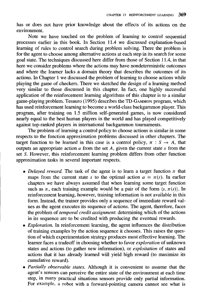
Partially observable states.
Although it is convenient to assume that the
agent's sensors can perceive the entire state of the environment at each time
step, in many practical situations sensors provide only partial information.
For example,
a
robot with a forward-pointing camera cannot see what is
behind it. In such cases, it may be necessary for the agent to consider its
previous observations together with its current sensor data when choosing
actions, and the best policy may be one that chooses actions specifically to
improve the observability of the environment.
Life-long learning.
Unlike isolated function approximation tasks, robot learn-
ing often requires that the robot learn several related tasks within the same
environment, using the same sensors. For example, a mobile robot may need
to learn how to dock on its battery charger, how to navigate through nar-
row corridors, and how to pick up output from laser printers. This setting
raises the possibility of using previously obtained experience or knowledge
to reduce sample complexity when learning new tasks.
13.2
THE LEARNING TASK
In this section we formulate the problem of learning sequential control strategies
more precisely. Note there are many ways to do so. For example, we might assume
the agent's actions are deterministic or that they are nondeterministic. We might
assume that the agent can predict the next state that will result from each action, or
that it cannot. We might assume that the agent is trained by an expert who shows
it examples of optimal action sequences, or that it must train itself by performing
actions of its own choice. Here we define one quite general formulation of the
problem, based on Markov decision processes. This formulation of the problem
follows the problem illustrated in Figure
13.1.
In
a
Markov decision process (MDP) the agent can perceive a set
S
of distinct
states of its environment and has a set
A
of actions that it can perform. At each
discrete time step
t,
the agent senses the current state
st,
chooses a current action
a,,
and performs it. The environment responds by giving the agent a reward
r,
=
r (st, a,)
and by producing the succeeding state
s,+l
=
6(s,,
a,).
Here the functions
6
and
r
are part of the environment and are not necessarily known to the agent.
In an MDP, the functions
6(st, a,)
and
r(s,, a,)
depend only on the current state
and action, and not on earlier states or actions. In this chapter we consider
only
the case in which
S
and
A
are finite. In general,
6
and
r
may be nondeterministic
functions, but we begin by considering only the deterministic case.
The task of the agent is to learn a
policy, n
:
S
+
A,
for selecting its next
action
a,
based on the current observed state
st;
that is,
n(s,)
=
a,.
How shall we
specify precisely which policy
n
we would like the agent to learn? One obvious
approach is to require the policy that produces the greatest possible cumulative
reward for the robot over time. To state this requirement more precisely, we define
the cumulative value
Vn(s,)
achieved by following an arbitrary policy
n
from an
arbitrary initial state
st
as follows:
CHAPTER
13
REINFORCEMENT
LEARNING
371
where the sequence of rewards rt+i is generated by beginning at state
s,
and by
repeatedly using the policy n to select actions as described above (i.e.,
a,
=
n(st),
a,+l
=
n(~,+~), etc.). Here
0
5
y
<
1 is a constant that determines the relative
value of delayed versus immediate rewards. In particular, rewards received
i
time
steps into the future are discounted exponentially by a factor of
y
'.
Note if we set
y
=
0,
only the immediate reward is considered. As we set
y
closer to 1, future
rewards are given greater emphasis relative to the immediate reward.
The quantity VX(s) defined by Equation (13.1) is often called the discounted
cumulative reward achieved by policy n from initial state s. It is reasonable to
discount future rewards relative to immediate rewards because, in many cases,
we prefer to obtain the reward sooner rather than later. However, other defini-
tions of total reward have also been explored. For example, jinite horizon reward,
c:=,
rt+i, considers the undiscounted sum of rewards over a finite number h of
.
-
steps. Another possibility is average reward,
limb,,
cF=~
rt+i, which consid-
ers the average reward per time step over the entire lifetime of the agent. In
this chapter we restrict ourselves to considering discounted reward as defined
by Equation (13.1). Mahadevan (1996) provides a discussion of reinforcement
learning when the criterion to be optimized is average reward.
We are now in a position to state precisely the agent's learning task. We
require that the agent learn a policy n that maximizes
V"(s) for all states s.
We will call such a policy an optimal policy and denote it by
T*.
n*
r
argmax V"
(s),
(Vs)
X
To simplify notation, we will refer to the value function v"*(s) of such an optimal
policy as V*(s). V*(s) gives the maximum discounted cumulative reward that the
agent can obtain starting from state s; that is, the discounted cumulative reward
obtained by following the optimal policy beginning at state s.
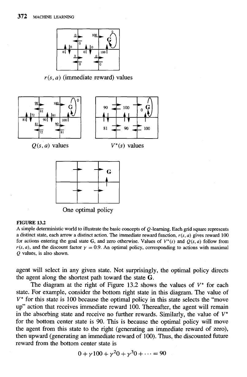
To illustrate these concepts, a simple grid-world environment is depicted
in the topmost diagram of Figure 13.2. The six grid squares in this diagram
represent six possible states, or locations, for the agent. Each arrow in the diagram
represents a possible action the agent can take to move from one state to another.
The number associated with each arrow represents the immediate reward
r(s, a)
the agent receives if it executes the corresponding state-action transition. Note
the immediate reward in this particular environment is defined to be zero for
all state-action transitions except for those leading into the state labeled
G.
It is
convenient to think of the state
G
as the goal state, because the only way the agent
can receive reward, in this case, is by entering this state. Note in this particular
environment, the only action available to the agent once it enters the state
G
is
to remain in this state. For this reason, we call
G
an absorbing state.
Once the states, actions, and immediate rewards are defined, and once we
choose a value for the discount factor
y,
we can determine the optimal policy n*
and its value function V*(s).
In
this case, let us choose
y
=
0.9. The diagram
at the bottom of the figure shows one optimal policy for this setting (there are
others as well). Like
any
policy, this policy specifies exactly one action that the
r
(s, a) (immediate reward) values
Q(s, a) values V*(s) values
One optimal policy
FIGURE
13.2
A simple deterministic world to illustrate the basic concepts of Q-learning. Each grid square represents
a distinct state, each arrow a distinct action. The immediate reward function,
r(s,
a)
gives reward 100
for actions entering the goal state
G,
and zero otherwise. Values of
V*(s)
and
Q(s,
a)
follow from
r(s,
a),
and the discount factor
y
=
0.9.
An optimal policy, corresponding to actions with maximal
Q values, is also shown.
agent will select in any given state. Not surprisingly, the optimal policy directs
the agent along the shortest path toward the state
G.
The diagram at the right of Figure 13.2 shows the values of V* for each
state. For example, consider the bottom right state in this diagram. The value of
V* for this state is 100 because the optimal policy in this state selects the "move
up" action that receives immediate reward 100. Thereafter, the agent will remain
in the absorbing state and receive no further rewards. Similarly, the value of
V*
for the bottom center state is 90. This is because the optimal policy will move
the agent from this state to the right (generating an immediate reward of zero),
then upward (generating an immediate reward of 100). Thus, the discounted future
reward from the bottom center state is
o+y100+y20+Y30+...=90
CHAPTER
13
REINFORCEMENT LEARNING
373
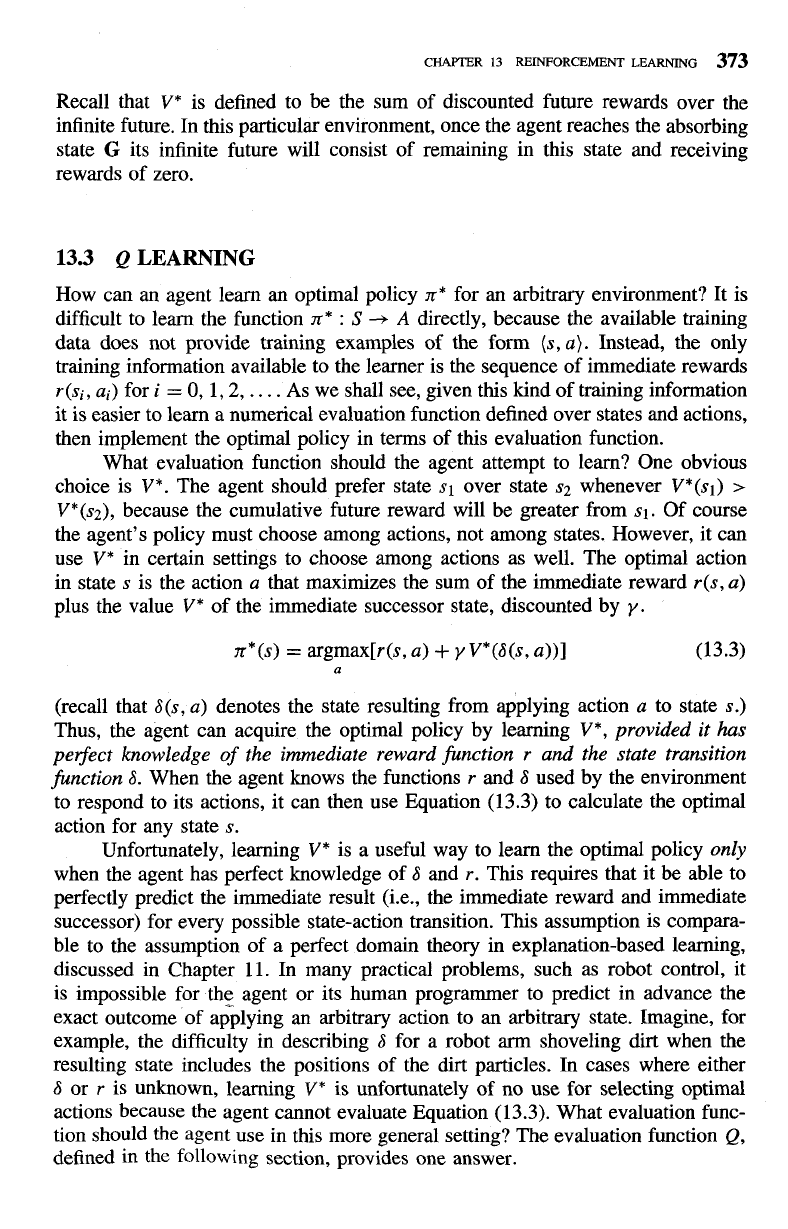
Recall that
V*
is defined to be the sum of discounted future rewards over the
infinite future. In this particular environment, once the agent reaches the absorbing
state
G
its infinite future will consist of remaining in this state and receiving
rewards of zero.
13.3
Q
LEARNING
How can an agent learn an optimal policy
n*
for an arbitrary environment? It is
difficult to learn the function
rt*
:
S
+
A
directly, because the available training
data does not provide training examples of the form
(s, a).
Instead, the only
training information available to the learner is the sequence of immediate rewards
r(si, ai)
for
i
=
0,
1,2,
. .
. .
As we shall see, given this kind of training information
it is easier to learn a numerical evaluation function defined over states and actions,
then implement the optimal policy in terms of this evaluation function.
What evaluation function should the agent attempt to learn? One obvious
choice is
V*.
The agent should prefer state
sl
over state
s2
whenever
V*(sl)
>
V*(s2),
because the cumulative future reward will be greater from
sl.
Of course
the agent's policy must choose among actions, not among states. However, it can
use
V*
in certain settings to choose among actions as well. The optimal action
in state
s
is the action
a
that maximizes the sum of the immediate reward
r(s, a)
plus the value
V*
of the immediate successor state, discounted by
y.
n*(s)
=
argmax[r(s, a)
f
y
V*(G(s, a))]
a
(recall that
6(s, a)
denotes the state resulting from applying action
a
to state
s.)
Thus, the agent can acquire the optimal policy by learning
V*,
provided it has
perfect knowledge
of
the immediate reward function
r
and the state transition
function
6.
When the agent knows the functions
r
and
6
used by the environment
to respond to its actions, it can then use Equation (13.3) to calculate the optimal
action for any state
s.
Unfortunately, learning
V*
is a useful way to learn the optimal policy only
when the agent has perfect knowledge of
6
and
r.
This requires that it be able to
perfectly predict the immediate result (i.e., the immediate reward
and
immediate
successor) for every possible state-action transition. This assumption is compara-
ble to the assumption of a perfect domain theory in explanation-based learning,
discussed in Chapter 11. In many practical problems, such as robot control, it
is impossible for the agent or its human programmer to predict in advance the
exact outcome of
applying an arbitrary action to an arbitrary state. Imagine, for
example, the difficulty in describing
6
for a robot
arm
shoveling dirt when the
resulting state includes the positions of the dirt particles. In cases where either
6
or
r
is unknown, learning
V*
is unfortunately of no use for selecting optimal
actions because the agent cannot evaluate Equation (13.3). What evaluation func-
tion should the agent use in this more general setting? The evaluation function
Q,
defined in the following section, provides one answer.
374
MACHINE LEARNING
13.3.1 The
Q
Function
Let us define the evaluation function
Q(s, a)
so that its value is the maximum dis-
counted cumulative reward that can be achieved starting from state
s
and applying
action
a
as the first action. In other words, the value of
Q
is the reward received
immediately upon executing action
a
from state
s,
plus the value (discounted by
y) of following the optimal policy thereafter.
Q(s, a)
-
r(s, a)
+
Y
V*(6(s, a))
(1
3.4)
Note that
Q(s, a)
is exactly the quantity that is maximized in Equation (13.3)
in order to choose the optimal action
a
in state
s.
Therefore, we can rewrite
Equation (13.3) in terms of
Q(s, a)
as
n
*
(s)
=
argmax
Q (s
,
a)
(13.5)
a
Why is this rewrite important? Because it shows that if the agent learns the
Q
function instead of the
V*
function, it will be able to select optimal actions
even
when it has no knowledge
of
thefunctions r and
6.
As Equation (13.5) makes clear,
it need only consider each available action
a
in its current state
s
and choose the
action that maximizes
Q(s, a).
It may at first seem surprising that one can choose globally optimal action
sequences by reacting repeatedly to the local values of
Q
for the current state.
This means the agent can choose the optimal action without ever conducting a
lookahead search to explicitly consider what state results from the action.
Part
of
the beauty of
Q
learning is that the evaluation function is defined to have precisely
this property-the value of
Q
for the current state and action summarizes in a
single number all the information needed to determine the discounted cumulative
reward that will be gained in the future if action
a
is selected in state
s.
To illustrate, Figure 13.2 shows the
Q
values for every state and action in the
simple grid world. Notice that the
Q
value for each state-action transition equals
the
r
value for this transition plus the
V*
value for the resulting state discounted by
y. Note also that the optimal policy shown in the figure corresponds to selecting
actions with maximal
Q
values.
13.3.2 An Algorithm for Learning
Q
Learning the
Q
function corresponds to learning the optimal policy. How can
Q
be learned?
The key problem is finding a reliable way to estimate training values for
Q,
given only a sequence of immediate rewards
r
spread out over time. This can
be accomplished through iterative approximation. To see how, notice the close
relationship between
Q
and
V*,
V*(S)
=
max
Q(s, a')
a'
which allows rewriting Equation
(13.4)
as
Q(s,
a)
=
r(s, a)
+
y max
Q(W, a), a')
a'
CHAPTER
13
REINFORCEMENT LEARNJNG
375
This recursive definition of Q provides the basis for algorithms that iter-
atively approximate Q (Watkins
1989).
To describe the algorithm, we will use
the symbol
Q
to refer to the learner's estimate, or hypothesis, of the actual
Q
function. In this algorithm the learner represents its hypothesis
Q
by
a
large table
with a separate entry for each state-action pair. The table entry for the pair (s, a)
stores the value for ~(s, a)-the learner's current hypothesis about the actual
but unknown value Q(s, a). The table can be initially filled with random values
(though it is easier to understand the algorithm if one assumes initial values of
zero). The agent repeatedly observes its current state s, chooses some action a,
executes this action, then observes the resulting reward r
=
r(s,
a)
and the new
state s'
=
6(s, a). It then updates the table entry for ~(s,
a)
following each such
transition, according to the rule:
Q(S, a)
t
r
+
y
max &(st, a')
a'
(13.7)
Note this training rule uses the agent's current
Q
values for the new state
s' to refine its estimate of ~(s, a) for the previous state s. This training rule
is motivated by Equation
(13.6), although the training rule concerns the agent's
approximation Q, whereas Equation (13.6) applies to the actual Q function. Note
although Equation (13.6) describes Q in terms of the functions 6(s, a) and r(s,
a),
the agent does not need to know these general functions to apply the training
rule of Equation (13.7). Instead it executes the action in its environment and
then observes the resulting new state
s' and reward r. Thus, it can be viewed as
sampling these functions at the current values of s and a.
The above Q learning algorithm for deterministic Markov decision processes
is described more precisely in Table 13.1. Using this algorithm the agent's estimate
Q
converges in the limit to the actual Q function, provided the system can be
modeled as a deterministic Markov decision process, the reward function r is
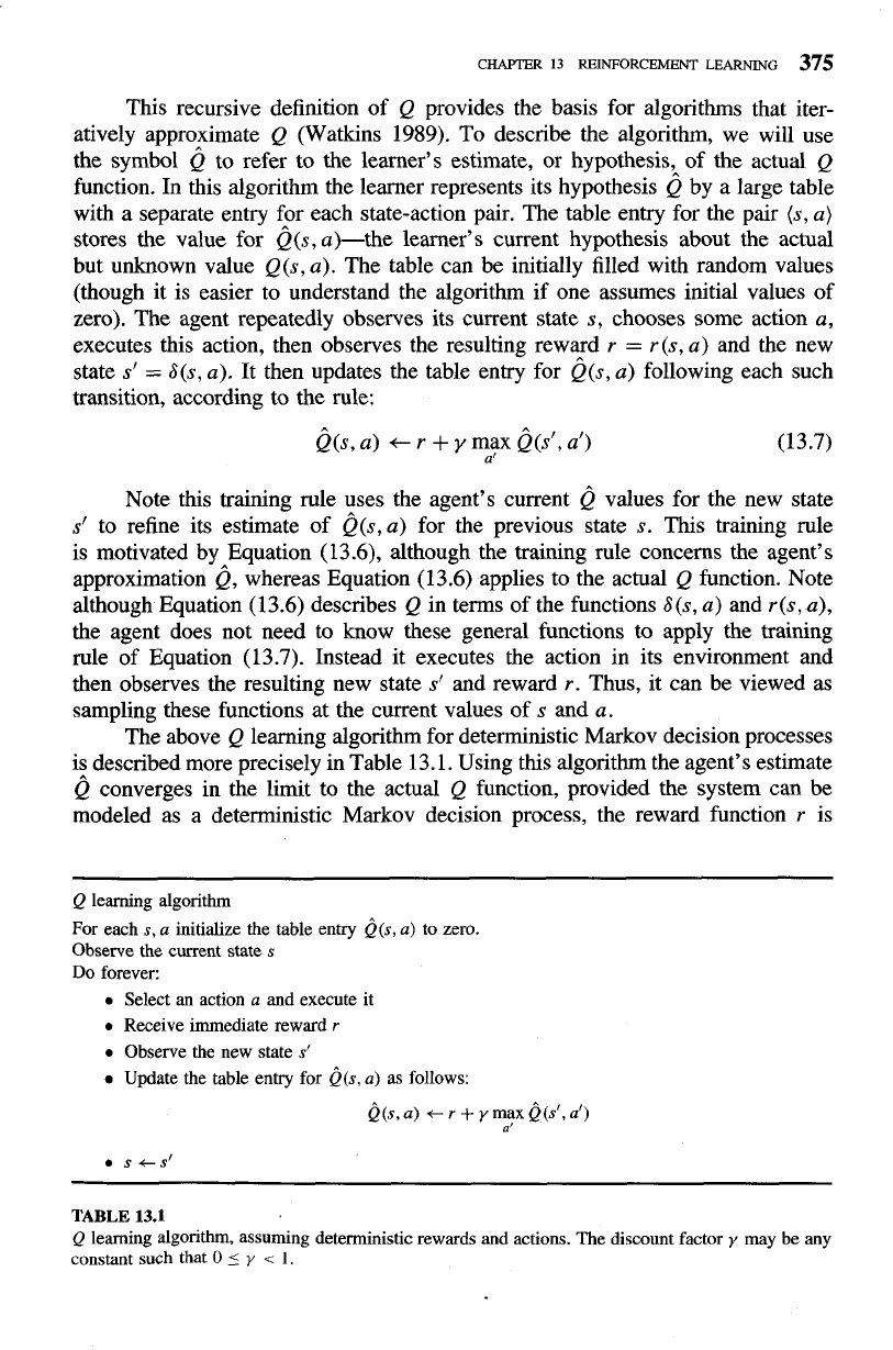
Q
learning algorithm
For each
s,
a initialize the table entry ~(s, a) to zero.
Observe
the
current state
s
Do forever:
Select an action a and execute it
Receive immediate reward
r
Observe the new state
s'
Update the table entry for
~(s,
a) as follows:
~(s,a)
cr
+
ymax&(s',af)
a'
S
CS'
TABLE
13.1
Q
learning algorithm, assuming deterministic rewards and actions. The discount factor y may be any
constant such that
0
5
y
<
1.
bounded, and actions are chosen so that every state-action pair is visited infinitely
often.
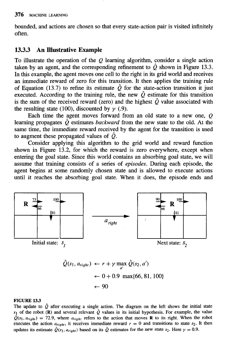
13.3.3
An
Illustrative Example
To illustrate the operation of the
Q
learning algorithm, consider a single action
taken by an agent, and the corresponding refinement to
Q
shown in Figure 13.3.
In
this example, the agent moves one cell to the right in its grid world and receives
an immediate reward of zero for this transition. It then applies the training rule
of Equation (13.7) to refine its estimate
Q
for the state-action transition it just
executed. According to the training rule, the new
Q
estimate for this transition
is the sum of the received reward (zero) and the highest
Q
value associated with
the resulting state (loo), discounted by
y
(.9).
Each time the agent moves forward from an old state to a new one,
Q
learning propagates
Q
estimates
backward
from the new state to the old. At the
same time, the immediate reward received by the agent for the transition is used
to augment these propagated values of
Q.
Consider applying this algorithm to the grid world and reward function
shown in Figure 13.2, for which the reward is zero everywhere, except when
entering the goal state. Since this world contains an absorbing goal state, we will
assume that training consists of a series of
episodes.
During each episode, the
agent begins at some randomly chosen state and is allowed to execute actions
until it reaches the absorbing goal state. When it does, the episode ends
and
Initial
state:
S]
Next state:
S2
FIGURE
13.3
The update to
Q
after executing a single^ action. The diagram on the left shows the initial state
s!
of the robot
(R)
and several relevant
Q
values in its initial hypothesis. For example, the value
Q(s1,
aright)
=
72.9, where
aright
refers to the action that moves
R
to its right. When the robot
executes the action
aright,
it receives immediate reward
r
=
0 and transitions to state
s2.
It then
updates its estimate
i)(sl,
aright)
based on its
Q
estimates for the new state
s2.
Here
y
=
0.9.
CHAPTER
13
REINFORCEMENT LEARNING
377
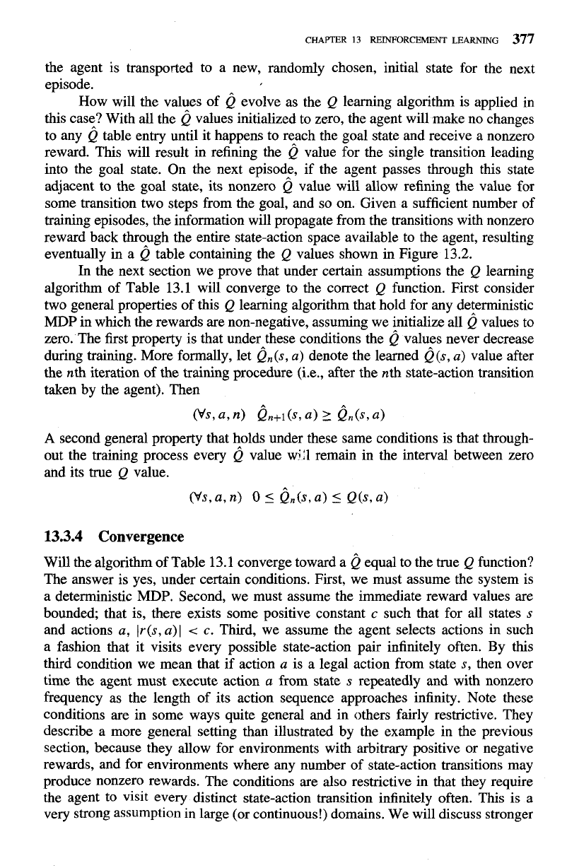
the agent is transported to a new, randomly chosen, initial state for the next
episode.
How will the values of
Q
evolve as the
Q
learning algorithm is applied in
this case? With all the
Q
values initialized to zero, the agent will make no changes
to any
Q
table entry until it happens to reach the goal state and receive a nonzero
reward. This will result in refining the
Q
value for the single transition leading
into the goal state. On the next episode, if the agent passes through this state
adjacent to the goal state, its nonzero
Q
value will allow refining the value for
some transition two steps from the goal, and so on. Given a sufficient number of
training episodes, the information will propagate from the transitions with nonzero
reward back through the entire state-action space available to the agent, resulting
eventually in a
Q
table containing the
Q
values shown in Figure 13.2.
In the next section we prove that under certain assumptions the
Q
learning
algorithm of Table 13.1 will converge to the correct
Q
function. First consider
two general properties of this
Q
learning algorithm that hold for any deterministic
MDP in which the rewards are non-negative, assuming we initialize all
Q
values to
zero. The first property is that under these conditions the
Q
values never decrease
during training. More formally, let Q,(s, a) denote the learned ~(s, a) value after
the nth iteration of the training procedure
(i.e., after the nth state-action transition
taken by the agent). Then
A
second general property that holds under these same conditions is that through-
out the training process every
Q
value wi:l remain in the interval between zero
and its true
Q
value.
13.3.4
Convergence
Will the algorithm of Table 13.1 converge toward a
Q
equal to the true
Q
function?
The answer is yes, under certain conditions. First, we must assume the system is
a deterministic MDP. Second, we must assume the immediate reward values are
bounded; that is, there exists some positive constant
c
such that for all states s
and actions a, Ir(s, a)l
<
c.
Third, we assume the agent selects actions in such
a fashion that it visits every possible state-action pair infinitely often. By this
third condition we mean that if action a is a legal action from state s, then over
time the agent must execute action a from state
s repeatedly and with nonzero
frequency as the length of its action sequence approaches infinity. Note these
conditions are in some ways quite general and in others fairly restrictive. They
describe a more general setting than illustrated by the example in the previous
section, because they allow for environments with arbitrary positive or negative
rewards, and for environments where any number of state-action transitions may
produce nonzero rewards. The conditions are also restrictive in that they require
the agent to visit
every
distinct state-action transition infinitely often. This is a
very strong assumption in large (or continuous!) domains. We will discuss stronger
convergence results later. However, the result described in this section provides
the basic intuition for understanding why
Q
learning works.
The key idea underlying the proof of convergence is that the table entry
~(s,
a)
with the largest error must have its error reduced by a factor of
y
whenever
it is updated. The reason is that its new value depends only in
part
on error-prone
Q
estimates, with the remainder depending on the error-free observed immediate
reward
r.
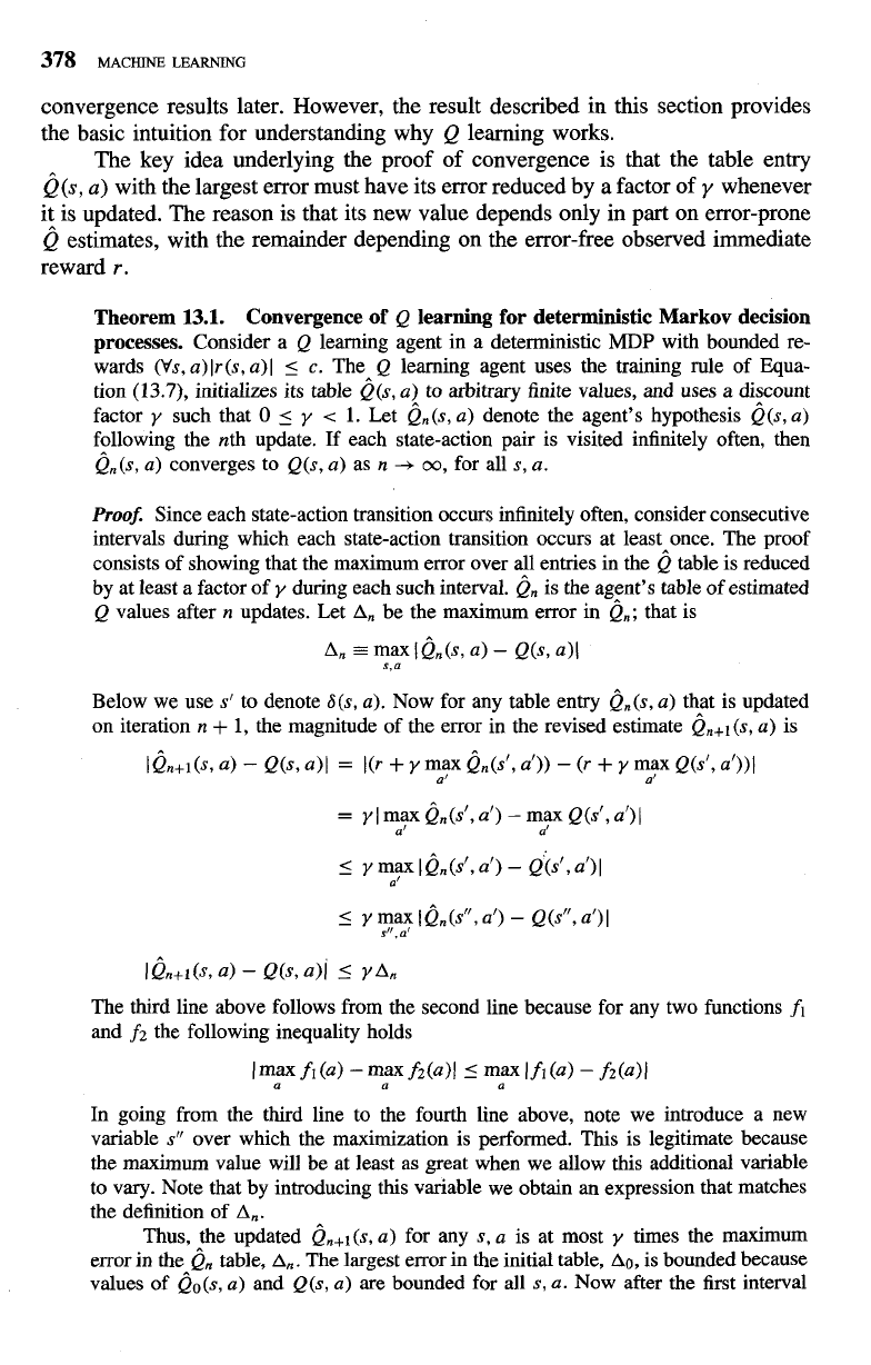
Theorem
13.1.
Convergence of
Q
learning for deterministic Markov decision
processes.
Consider a
Q
learning agent in a deterministic
MDP
with bounded re-
wards
(Vs, a) lr(s, a)[
5
c.
The*
Q
learning agent uses the training rule of Equa-
tion
(13.7),
initializes its table
Q(s, a)
to arbitrary finite values, and uses a discount
factor
y
such that
0
y
<
1.
Let
Q,(s, a)
denote the agent's hypothesis
~(s, a)
following the nth update.
If
each state-action pair is visited infinitely often, then
Q,(s,
a)
converges to
Q(s, a)
as n
+
oo,
for all
s, a.
Proof.
Since each state-action transition occurs infinitely often, consider consecutive
intervals during which each state-action transition occurs at least once. The proof
consists of showing that the maximum error over all entries in the
Q
table is reduced
by at least a factor of
y
during each such interval.
Q,
is the agent's table of estimated
Q
values after n updates. Let
An
be the maximum error in
Q,;
that is
Below we use
s'
to denote
S(s, a).
Now for any table entry
(in@,
a)
that is updated
on iteration n
+
1,
the magnitude of the error in the revised estimate
Q,+~(S,
a)
is
IQ,+I(S, a)
-
Q(s, all
=
I(r
+
y
max
Qn(s', a'))
-
(r
+
y
m?x
Q(d, a'))]
a' a
=
y
I
my
Qn(st, a')
-
my
Q(s1, a')
I
a a
5
y
max
I
Qn(s1, a')
-
~(s', a')
I
a'
5
Y
my
I
Q, (s", a')
-
QW, a')
I
s
,a
I
Qn+i
(s,
a)
-
Q(s, all
5
Y
An
The third line above follows from the second line because for any two functions
fi
and
f2
the following inequality holds
In going from the third line to the fourth line above, note we introduce a new
variable
s"
over which the maximization is performed. This is legitimate because
the maximum value will be at least as great when we allow this additional variable
to vary. Note that by introducing this variable we obtain an expression that matches
the definition of
A,.
Thus, the updated
Q,+~(S,
a)
for any
s,
a
is at most
y
times the maximum
error in the
Q,,
table,
A,.
The largest error in the initial table,
Ao,
is bounded because
values of
~~(s, a)
and
Q(s, a)
are bounded for all
s, a.
Now after the first interval