Mitchell Т. Machine learning

Подождите немного. Документ загружается.

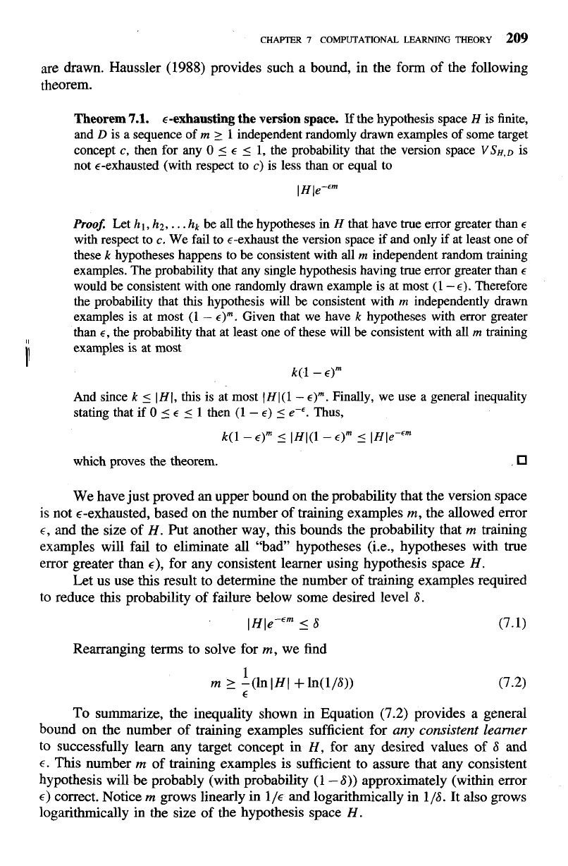
are drawn. Haussler (1988) provides such a bound, in the form of the following

theorem.

Theorem

7.1.

€-exhausting the version space. If the hypothesis space

is finite,

and

is a sequence of

1 independent randomly drawn examples of some target

concept c, then for any

1, the probability that the version space

VSH,~

not €-exhausted (with respect to c) is less than or equal to

Proof.

Let

hl, h2,

. . .

be all the hypotheses in

that have true error greater than

with respect to c. We fail to €-exhaust the version space if and only if at least one of

these

hypotheses happens to be consistent with all

independent random training

examples. The probability that any single hypothesis having true error greater than

would be consistent with one randomly drawn example is at most (1

E).

Therefore

the probability that this hypothesis will

consistent with

independently drawn

examples is at most (1

E)~. Given that we have

hypotheses with error greater

than E, the probability that at least one of these will be consistent with all

training

examples is at most

And since

this is at most

I(1-

6)".

Finally, we use a general inequality

stating that if

1 then (1

e-'.

Thus,

which proves the theorem.

We have just proved an upper bound on the probability that the version space

is not €-exhausted, based on the number of training examples

the allowed error

E, and the size of

Put another way, this bounds the probability that

training

examples will fail to eliminate all "bad" hypotheses (i.e., hypotheses with true

error greater than

E),

for any consistent learner using hypothesis space

Let us use this result to determine the number of training examples required

to reduce this probability of failure below some desired level 6.

Rearranging terms to solve for

we find

(ln

ln(l/6))

(7.2)

To summarize, the inequality shown in Equation (7.2) provides a general

bound on the number of training examples sufficient for

any consistent learner

to successfully learn any target concept in

for any desired values of 6 and

E. This number

of training examples is sufficient to assure that any consistent

hypothesis will be probably (with probability

6)) approximately (within error

E) correct. Notice

grows linearly in 1/~ and logarithmically in 116. It also grows

logarithmically in the size

the hypothesis space

210

MACHINE

LEARNING

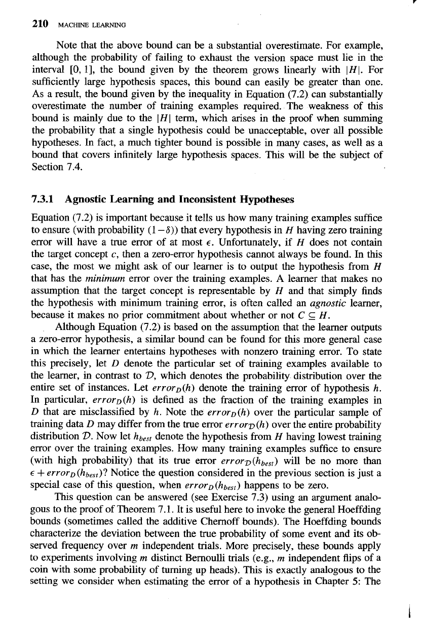
Note that the above bound can be a substantial overestimate. For example,

although the probability of failing to exhaust the version space must lie in the

interval

[O,

11, the bound given by the theorem grows linearly with

IHI.

For

sufficiently large hypothesis spaces, this bound can easily be greater than one.

As a result, the bound given by the inequality in Equation (7.2) can substantially

overestimate the number of training examples required. The weakness of this

bound is mainly due to the

IHI

term, which arises in the proof when summing

the probability that a single hypothesis could be unacceptable, over all possible

hypotheses. In fact, a much tighter bound is possible in many cases, as well as a

bound that covers infinitely large hypothesis spaces. This will be the subject of

Section 7.4.

7.3.1

Agnostic Learning and Inconsistent Hypotheses

Equation (7.2) is important because it tells us how many training examples suffice

to ensure (with probability (1

6))

that every hypothesis in

having zero training

error will have a true error of at most

Unfortunately, if

does not contain

the target concept

then a zero-error hypothesis cannot always be found. In this

case, the most we might ask of our learner is to output the hypothesis from

that has the minimum error over the training examples. A learner that makes no

assumption that the target concept is representable by

and that simply finds

the hypothesis with minimum training error, is often called an agnostic learner,

because it makes no prior commitment about whether or not

Although Equation (7.2) is based on the assumption that the learner outputs

a zero-error hypothesis, a similar bound can be found for this more general case

in which the learner entertains hypotheses with nonzero training error. To state

this precisely, let

denote the particular set of training examples available to

the learner, in contrast to

which denotes the probability distribution over the

entire set of instances. Let errorD(h) denote the training error of hypothesis h.

In particular, error~(h) is defined as the fraction of the training examples in

that are misclassified by h. Note the errorD(h) over the particular sample of

training data

may differ from the true error errorv(h) over the entire probability

distribution

2).

Now let hb,,, denote the hypothesis from

having lowest training

error over the training examples. How many training examples suffice to ensure

(with high probability) that its true error errorD(hb,,,) will be no more than

errorg (hbest)? Notice the question considered in the previous section is just a

special case of this question, when errorD(hb,,) happens to

zero.

This question can be answered (see Exercise 7.3) using an argument analo-

gous to the proof of Theorem 7.1. It is useful here to invoke the general Hoeffding

bounds (sometimes called the additive Chernoff bounds). The Hoeffding bounds

characterize the deviation between the true probability of some event and its ob-

served frequency over

independent trials. More precisely, these bounds apply

to experiments involving

distinct Bernoulli trials (e.g.,

independent flips of a

coin with some probability of turning up heads). This is exactly analogous to the

setting we consider when estimating the error of a hypothesis in Chapter

The

CHAPTER

COMPUTATIONAL LEARNING THEORY

211

probability of the coin being heads corresponds to the probability that the hypothe-

sis will misclassify a randomly drawn instance. The

independent coin flips corre-

spond to the

independently drawn instances. The frequency of heads over the

examples corresponds to the frequency of misclassifications over the

instances.

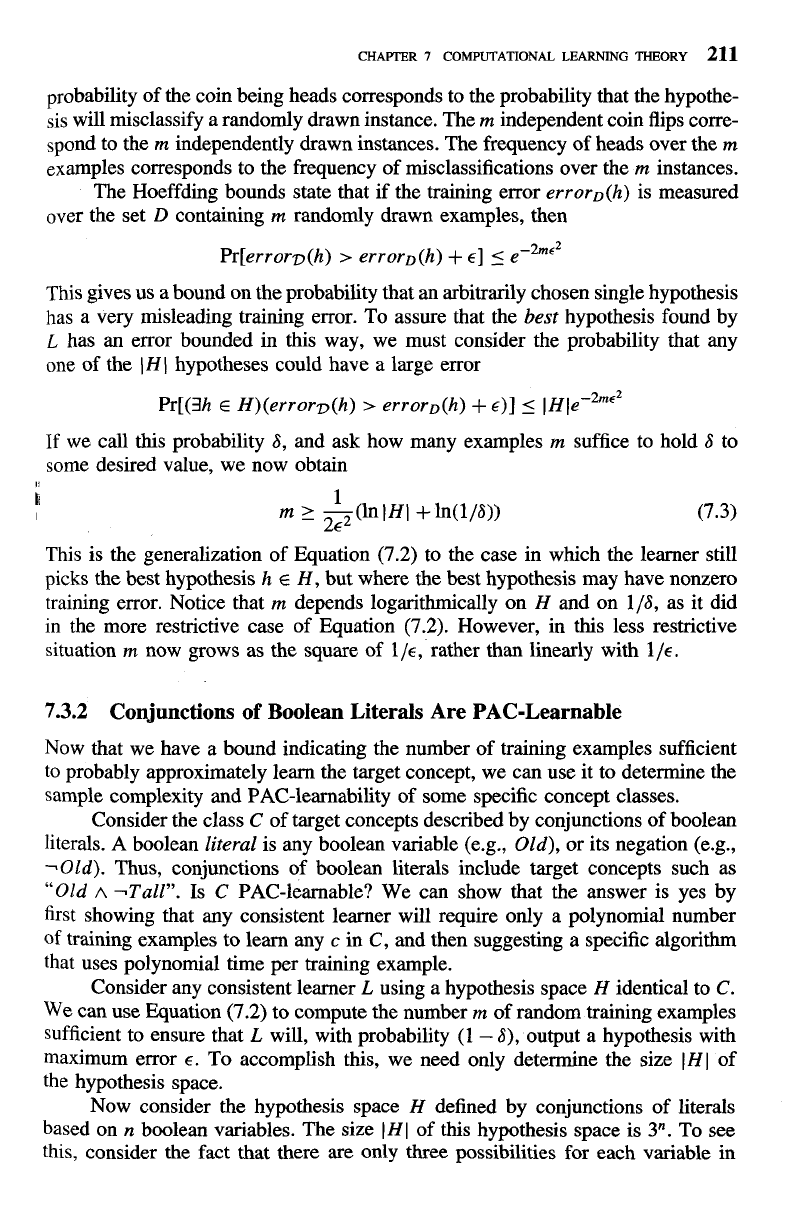
The Hoeffding bounds state that if the training error errOrD(h) is measured

over the set

containing

randomly drawn examples, then

This gives us a bound on the probability that an arbitrarily chosen single hypothesis

has a very misleading training error. To assure that the best hypothesis found by

has an error bounded in this way, we must consider the probability that any

one of the

hypotheses could have a large error

Pr[(3h

H)(errorv(h)

error~(h)

E)]

~e-~~'~

call this probability

and ask how many examples

suffice to hold

some desired value, we now obtain

This is the generalization of Equation

(7.2)

to the case in which the learner still

picks the best hypothesis h

H, but where the best hypothesis may have nonzero

training error. Notice that

depends logarithmically on H and on 116, as it did

in the more restrictive case of Equation (7.2). However, in this less restrictive

situation

now grows as the square of 116, rather than linearly with 116.

7.3.2

Conjunctions of Boolean Literals Are PAC-Learnable

Now that we have a bound indicating the number of training examples sufficient

to probably approximately learn the target concept, we can use it to determine the

sample complexity and PAC-learnability of some specific concept classes.

Consider the class

of target concepts described by conjunctions of boolean

literals.

boolean literal is any boolean variable (e.g., Old), or its negation (e.g.,

-Old). Thus, conjunctions of boolean literals include target concepts such as

"Old

-Tallv. Is

PAC-learnable? We can show that the answer is yes by

first showing that any consistent learner will require only a polynomial number

training examples to learn any

and then suggesting a specific algorithm

that uses polynomial time per training example.

Consider any consistent learner

using a hypothesis space H identical to

We can use Equation (7.2) to compute the number

of random training examples

sufficient to ensure that

will, with probability (1

S), output a hypothesis with

maximum error

To accomplish this, we need only determine the size IHI of

the hypothesis space.

Now consider the hypothesis space H defined by conjunctions of literals

based on

boolean variables. The size 1HI of this hypothesis space is

3".

To see

this, consider the fact that there are only three possibilities for each variable in

212

MACHINE

LEARNING

any given hypothesis: Include the variable as a literal in the hypothesis, include

its negation as a literal, or ignore it. Given

such variables, there are

distinct

hypotheses.

Substituting

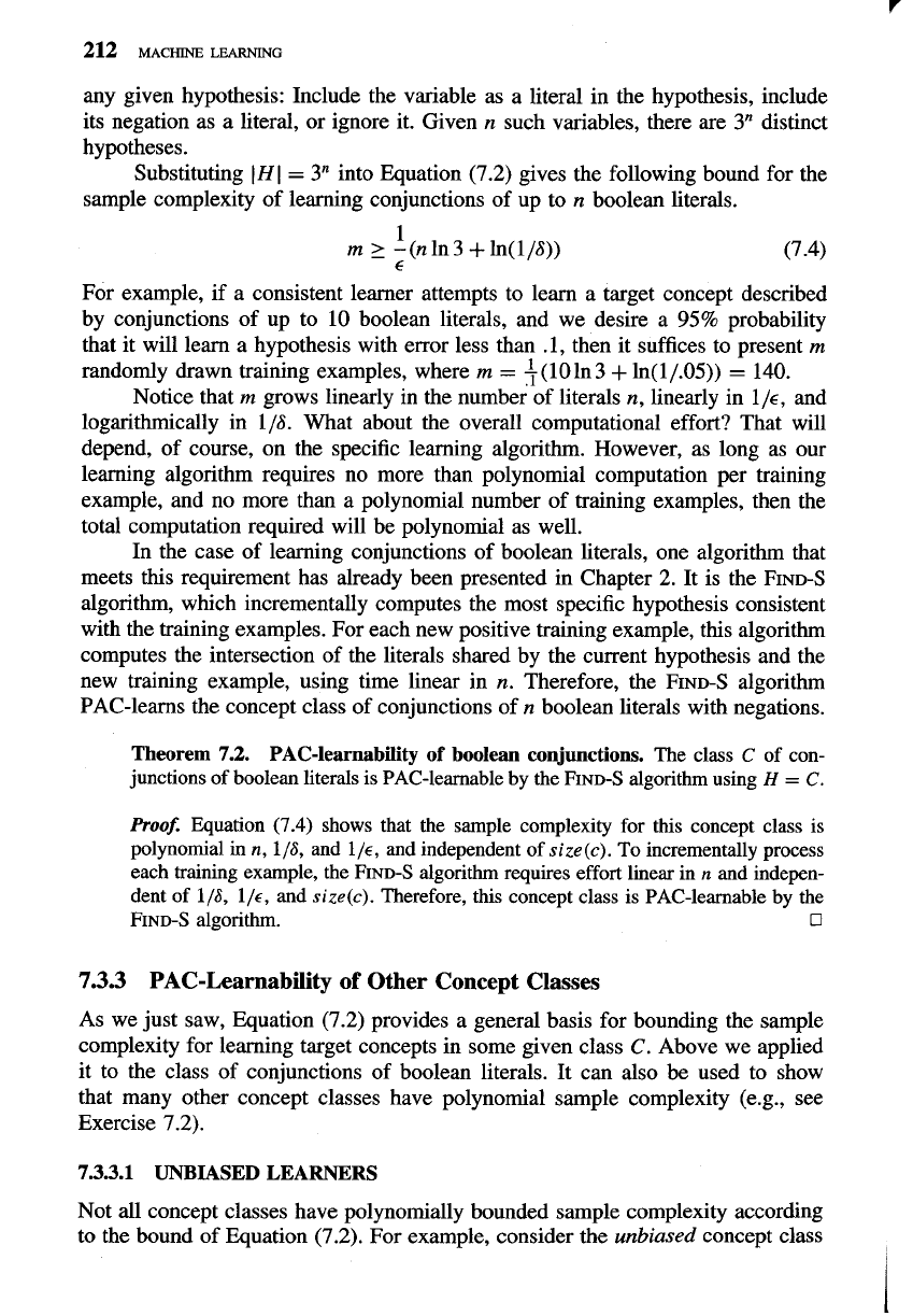
into Equation (7.2) gives the following bound for the

sample complexity of learning conjunctions of up to

boolean literals.

For example, if a consistent learner attempts to learn a target concept described

by conjunctions of up to 10 boolean literals, and we desire a

95%

probability

that it will learn a hypothesis with error less than .l, then it suffices to present

randomly drawn training examples, where

(10 1n

ln(11.05))

140.

Notice that

grows linearly in the number of literals

linearly in 116, and

logarithmically in 116. What about the overall computational effort? That will

depend, of course, on the specific learning algorithm. However, as long as our

learning algorithm requires no more than polynomial computation per training

example, and no more than

polynomial number of training examples, then the

total computation required will be polynomial as well.

In the case of learning conjunctions of boolean literals, one algorithm that

meets this requirement has already been presented in Chapter 2. It is the

FIND-S

algorithm, which incrementally computes the most specific hypothesis consistent

with the training examples. For each new positive training example, this algorithm

computes the intersection of the literals shared by the current hypothesis and the

new training example, using time linear in

Therefore, the

FIND-S

algorithm

PAC-learns the concept class of conjunctions of

boolean literals with negations.

Theorem

7.2.

PAC-learnability of boolean conjunctions.

The class C of con-

junctions of boolean literals is PAC-learnable by the FIND-S algorithm using

Proof.

Equation (7.4) shows that the sample complexity for this concept class is

polynomial in

116,

and

116,

and independent of

size (c).

To incrementally process

each training example, the FIND-S algorithm requires effort linear in

and indepen-

dent of

116, 116,

and

size(c).

Therefore, this concept class is PAC-learnable by the

FIND-S algorithm.

7.3.3

PAC-Learnability of Other Concept Classes

As we just saw, Equation (7.2) provides a general basis for bounding the sample

complexity for learning target concepts in some given class

Above we applied

it to the class of conjunctions of boolean literals. It can also be used to show

that many other concept classes have polynomial sample complexity (e.g., see

Exercise 7.2).

7.3.3.1

UNBIASED

LEARNERS

Not all concept classes have polynomially bounded sample complexity according

to the bound of Equation (7.2). For example, consider the

unbiased

concept class

that contains every teachable concept relative to

The set C of all definable

target concepts corresponds to the power set of X-the set of all subsets of

X-

which contains ICI

2IXI concepts. Suppose that instances in X are defined by

boolean features. In this case, there will be

1x1

2" distinct instances, and

therefore ICI

21'1

2' distinct concepts. Of course to learn such an unbiased

concept class, the learner must itself use an unbiased hypothesis space H

Substituting

22n into Equation (7.2) gives the sample complexity for learning

the unbiased concept class relative to

Thus, this unbiased class of target concepts has exponential sample complexity

under the PAC model, according to Equation (7.2). Although Equations (7.2)

and (7.5) are not tight upper bounds, it can in fact

proven that the sample

complexity for the unbiased concept class is exponential in

7.3.3.2

K-TERM DNF

AND

K-CNF CONCEPTS

It is also possible to find concept classes that have polynomial sample complexity,

but nevertheless cannot be learned in polynomial time. One interesting example is

the concept class C of k-term disjunctive normal form (k-term DNF) expressions.

k-term DNF expressions are of the form

. .

Tk, where each term

1;:

is a conjunction of

boolean attributes and their negations. Assuming H

is easy to show that

HI is at most 3"k (because there are k terms, each of which

may take on

possible values). Note 3"k is an overestimate of H, because it is

double counting the cases where

I;.

and where

1;:

more_general-than

I;..

Still, we can use this upper bound on

HI to obtain an upper bound on the sample

complexity, substituting this into Equation (7.2).

which indicates that the sample complexity of k-term DNF is polynomial in

1/~,

116,

and k. Despite having polynomial sample complexity, the computa-

tional complexity is not polynomial, because this learning problem can be shown

to be equivalent to other problems that are known to be unsolvable in polynomial

time (unless RP

NP). Thus, although k-term DNF has polynomial sample

complexity, it does not have polynomial computational complexity for a learner

using H

The surprising fact about k-term DNF is that although it is not PAC-

learnable, there is a strictly larger concept class that is! This is possible because

the larger concept class has polynomial computation complexity per example and

still has polynomial sample complexity. This larger class is the class of k-CNF

expressions: conjunctions of arbitrary length of the form

. .

I;.,

where

each is a disjunction of up to k boolean attributes. It is straightforward to show

that k-CNF subsumes k-DNF, because any k-term DNF expression can easily be

rewritten as a k-CNF expression (but not vice versa). Although k-CNF is more

expressive than k-term DNF, it has both polynomial sample complexity and poly-

nomial time complexity. Hence, the concept class k-term DNF is PAC learnable

by an efficient algorithm using H

k-CNF. See Kearns and Vazirani (1994) for

a more detailed discussion.

7.4 SAMPLE COMPLEXITY FOR INFINITE HYPOTHESIS SPACES

In the above section we showed that sample complexity for PAC learning grows

as the logarithm of the size of the hypothesis space. While Equation (7.2) is quite

useful, there are two drawbacks to characterizing sample complexity in terms of

IHI. First, it can lead to quite weak bounds (recall that the bound on

can be

significantly greater than 1 for large

H I). Second, in the case of infinite hypothesis

spaces we cannot apply Equation (7.2) at all!

Here we consider a second measure of the complexity of H, called the

Vapnik-Chervonenkis dimension of H (VC dimension, or VC(H), for short). As

we shall see, we can state bounds on sample complexity that use VC(H) rather

than

IHI. In many cases, the sample complexity bounds based on VC(H) will

be tighter than those from Equation (7.2). In addition, these bounds allow us to

characterize the sample complexity of many infinite hypothesis spaces, and can

be shown to be fairly tight.

7.4.1 Shattering a Set

Instances

The VC dimension measures the complexity of the hypothesis space H, not by the

number of distinct hypotheses

but instead by the number of distinct instances

from

that can be completely discriminated using H.

To make this notion more precise, we first define the notion of

shattering

set of instances. Consider some subset of instances S

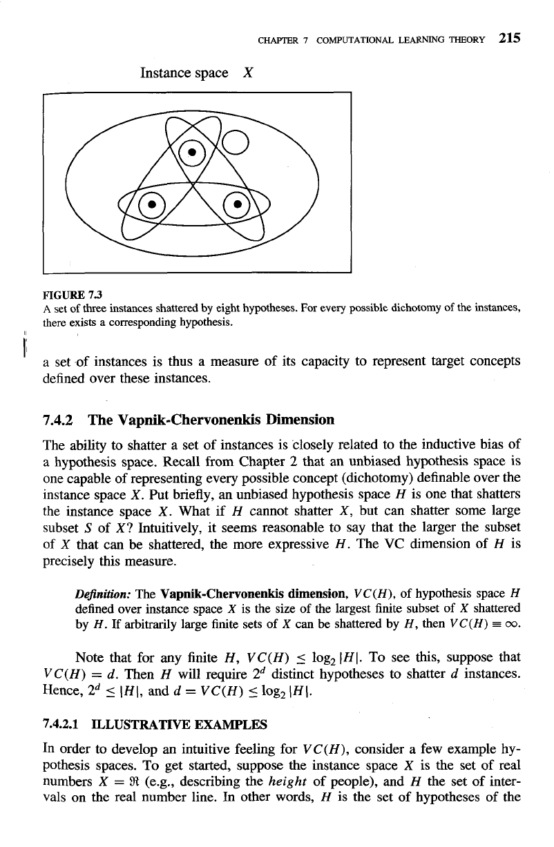
For example, Figure 7.3

shows a subset of three instances from

Each hypothesis h from H imposes some

dichotomy on S; that is, h partitions S into the two subsets {x

Slh(x)

1) and

Slh(x)

0).

Given some instance set S, there are 2ISI possible dichotomies,

though H may be unable to represent some of these. We say that H shatters S if

every possible dichotomy of

S can be represented by some hypothesis from H.

Definition:

set of instances

shattered

by hypothesis space

if and only if

for every dichotomy.of

there exists some hypothesis in

consistent with this

dichotomy.

Figure 7.3 illustrates a set S of three instances that is shattered by the

hypothesis space. Notice that each of the 23 dichotomies of these three instances

is covered by some hypothesis.

Note that if a set of instances is not shattered by a hypothesis space, then

there must be some concept (dichotomy) that can be defined over the instances,

but that cannot

represented by the hypothesis space. The ability

to shatter

Instance space

FIGURE

set

three instances shattered

eight hypotheses.

For

every

possible

dichotomy of

the instances,

there exists a corresponding hypothesis.

a set .of instances is thus a measure of its capacity to represent target concepts

defined over these instances.

7.4.2

The Vapnik-Chervonenkis Dimension

The ability to shatter a set of instances is closely related to the inductive bias of

hypothesis space. Recall from Chapter

that an unbiased hypothesis space is

one capable of representing every possible concept (dichotomy) definable over the

instance space

Put briefly, an unbiased hypothesis space H is one that shatters

the instance space

What if H cannot shatter

but can shatter some large

subset

Intuitively, it seems reasonable to say that the larger the subset

that can be shattered, the more expressive H. The VC dimension of H is

precisely this measure.

Definition:

The

Vapnik-Chervonenkis dimension,

VC(H),

of hypothesis space

defined over instance space

is the size of the largest finite subset of

shattered

arbitrarily large finite sets of

can be shattered by

then

VC(H)

oo.

Note that for any finite

VC(H)

log2 IHI. To see this, suppose that

VC(H)

Then H will require

distinct hypotheses to shatter

instances.

Hence,

IHI, andd

VC(H) slog2(H(.

7.4.2.1

ILLUSTRATIW

EXAMPLES

In order to develop an intuitive feeling for VC(H), consider a few example hy-

pothesis spaces. To get started, suppose the instance space

is the set of real

numbers

(e.g., describing the

height

of people), and H the set of inter-

vals on the real number line. In other words,

is the set of hypotheses of the

form

where

and

may be any real constants. What is VC(H)?

To answer this question, we must find the largest subset of

that can be shat-

tered by

Consider a particular subset containing two distinct instances, say

{3.1,5.7}. Can

be shattered by H? Yes. For example, the four hypotheses

2), (1

4),

7), and (1

7) will do. Together, they

represent each of the four dichotomies over

covering neither instance, either

one of the instances, and both of the instances, respectively. Since we have found

a set of size two that can be shattered by

we know the VC dimension of

is at least two. Is there a set of size three that can be shattered? Consider a set

(xo, xl, x2}

containing three arbitrary instances. Without loss of generality,

assume

x2.

Clearly this set cannot be shattered, because the dichotomy

that includes

and

x2,

but not

XI,

cannot be represented by a single closed inter-

val. Therefore,

subset

of size three can be shattered, and VC(H)

2. Note

here that H is infinite, but VC(H) finite.

Next consider the set

of instances corresponding to points on the

plane

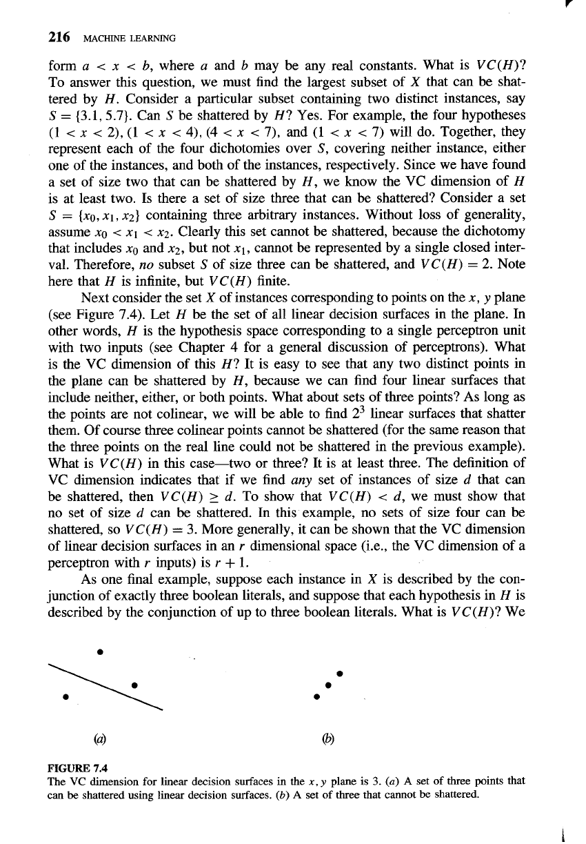
(see Figure 7.4). Let

be the set of all linear decision surfaces in the plane.

other words, H is the hypothesis space corresponding to a single perceptron unit

with two inputs (see Chapter 4 for a general discussion of perceptrons). What

is the VC dimension of this H? It is easy to see that any two distinct points in

the plane can be shattered by H, because we can find four linear surfaces that

include neither, either, or both points. What about sets of three points? As long as

the points are not colinear, we will be able to find

23 linear surfaces that shatter

them. Of course three colinear points cannot be shattered (for the same reason that

the three points on the real line could not be shattered in the previous example).

What is

VC(H) in this case-two or three? It is at least three. The definition of

VC dimension indicates that if we find

any

set of instances of size

that can

be shattered, then VC(H)

To show that VC(H)

we must show that

no set of size

can be shattered. In this example, no sets of size four can be

shattered, so VC(H)

3. More generally, it can be shown that the VC dimension

of linear decision surfaces in an

dimensional space (i.e., the VC dimension of a

perceptron with

inputs) is

As one final example, suppose each instance in

is described by the con-

junction of exactly three boolean literals, and suppose that each hypothesis in H is

described by the conjunction of up to three boolean literals. What is VC(H)? We

FIGURE

7.4

The

dimension for linear decision surfaces in the

plane is

(a)

set of three points that

can

shattered using linear decision surfaces.

(b)

set of three that cannot be shattered.

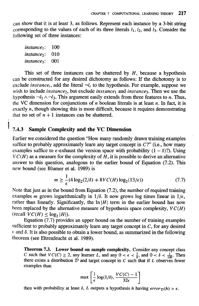
can show that it is at least 3, as follows. Represent each instance by a 3-bit string

corresponding to the values of each of its three literals 11, 12, and 13. Consider the

following set of three instances:

This set of three instances can be shattered by H, because a hypothesis

can be constructed for any desired dichotomy as follows: If the dichotomy is to

exclude instancei, add the literal

-li to the hypothesis. For example, suppose we

wish to include instance2, but exclude instance1 and instance3. Then we use the

hypothesis -Il

-I3. This argument easily extends from three features to

Thus,

the

dimension for conjunctions of n boolean literals is at least n. In fact, it is

exactly n, though showing this is more difficult, because it requires demonstrating

that no set of n

1 instances can be shattered.

7.4.3

Sample Complexity and the

Dimension

Earlier we considered the question "How many randomly drawn training examples

suffice to probably approximately learn any target concept in C?' (i.e., how many

examples suffice to €-exhaust the version space with probability (1

a)?). Using

VC(H) as a measure for the complexity of H, it is possible to derive an alternative

answer to this question, analogous to the earlier bound of Equation (7.2). This

new bound (see Blumer et

al.

1989) is

Note that just as in the bound from Equation (7.2), the number of required training

examples

grows logarithmically in 118. It now grows log times linear in 116,

rather than linearly. Significantly, the In

HI term in the earlier bound has now

been replaced by the alternative measure of hypothesis space complexity, VC(H)

(recall VC(H)

log2

H I).

Equation (7.7) provides an upper bound on the number of training examples

sufficient to probably approximately learn any target concept in C, for any desired

and

It is also possible to obtain a lower bound, as summarized in the following

theorem (see Ehrenfeucht et al. 1989).

Theorem

7.3.

Lower bound on sample complexity. Consider any concept class

such that

VC(C)

any learner

and

any

and

Then

there exists a distribution

and target concept in

such that if

observes fewer

examples than

then with probability at least

outputs a hypothesis

having

errorD(h)

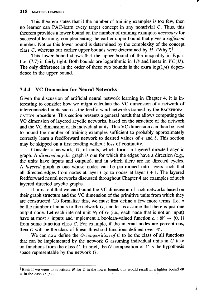
This theorem states that if the number of training examples is too few, then

no learner can PAC-learn every target concept in any nontrivial

Thus, this

theorem provides a lower bound on the number of training examples necessary for

successful learning, complementing the earlier upper bound that gives a

suficient

number. Notice this lower bound is determined by the complexity of the concept

class

whereas our earlier upper bounds were determined by

(why?)+

This lower bound shows that the upper bound of the inequality in Equa-

tion (7.7) is fairly tight. Both bounds are logarithmic in 116 and linear in

VC(H).

The only difference in the order of these two bounds is the extra log(l/c) depen-

dence in the upper bound.

7.4.4

Dimension for Neural Networks

Given the discussion of artificial neural network learning in Chapter

it is in-

teresting to consider how we might calculate the VC dimension of a network of

interconnected units such as the feedforward networks trained by the

BACKPROPA-

GATION

procedure. This section presents a general result that allows computing the

VC dimension of layered acyclic networks, based on the structure of the network

and the VC dimension of its individual units. This VC dimension can then be used

to bound the number of training examples sufficient to probably approximately

correctly learn a feedforward network to desired values of c and 6. This section

may be skipped on a first reading without loss of continuity.

Consider a network, G, of units, which forms a layered directed acyclic

graph.

directed acyclic graph is one for which the edges have a direction (e.g.,

the units have inputs and outputs), and in which there are no directed cycles.

A layered graph is one whose nodes can be partitioned into layers such that

all directed edges from nodes at layer 1 go to nodes at layer 1

1. The layered

feedforward neural networks discussed throughout Chapter

are examples of such

layered directed acyclic graphs.

It turns out that we can bound the VC dimension of such networks based on

their graph structure and the VC dimension of the primitive units from which they

are constructed. To formalize this, we must first define a few more terms. Let

be the number of inputs to the network G, and let us assume that there is just one

output node. Let each internal unit

of G (i.e., each node that is not an input)

have at most

inputs and implement a boolean-valued function

8''

(0,

from some function class

For example, if the internal nodes are perceptrons,

then

will be the class of linear threshold functions defined over

8'.

We can now define the G-composition of

to be the class of all functions

that can be implemented by the network G assuming individual units in

take

on functions from the class

In brief, the G-composition of

is the hypothesis

space representable by the network G.

t~int:

we were to substitute

for

in the lower bound, this would result in a tighter bound on

in the case