Mitchell Т. Machine learning

Подождите немного. Документ загружается.

CHAPTER

BAYESIAN LEARNING

189

For example, to calculate the derivative of In

P(D1h)

with respect to the upper-

rightmost entry in the table of Figure

6.3

we will have to calculate the quan-

tity

P(Campf ire

True, Storm

False, BusTourGroup

Falseld)

for each

training example

When these variables are unobservable for the training

example

this required probability can be calculated from the observed variables

using standard Bayesian network inference. In fact, these required quantities

are easily derived from the calculations performed during most Bayesian network

inference, so learning can be performed at little additional cost whenever the

Bayesian network is used for inference and new evidence is subsequently obtained.

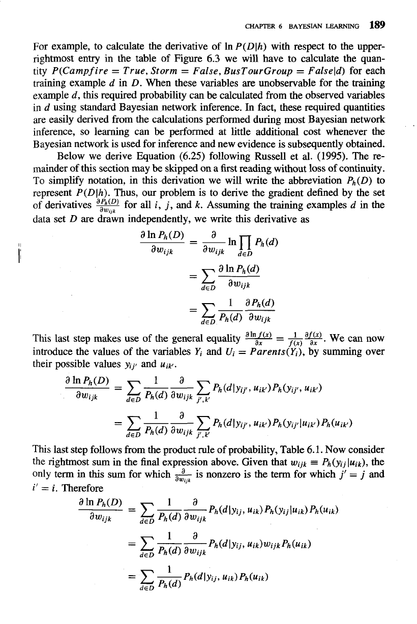
Below we derive Equation

(6.25)

following Russell et al.

(1995).

The re-

mainder of this section may be skipped on a first reading without loss of continuity.

To simplify notation, in this derivation we will write the abbreviation

Ph(D)

represent

P(DJh).

Thus, our problem is to derive the gradient defined by the set

derivatives for all

and

Assuming the training examples

the

data set

are drawn independently, we write this derivative as

This last step makes use of the general equality

f(~)

can

now

introduce the values of the variables

and

Parents(Yi),

by summing over

their possible values

yijl

and

uiu.

This last step follows from the product rule of probability, Table

6.1.

Now consider

the rightmost sum in the final expression above. Given that

Wijk

Ph(yijl~ik),

the

only term

this sum for which

is nonzero is the term for which

and

Therefore

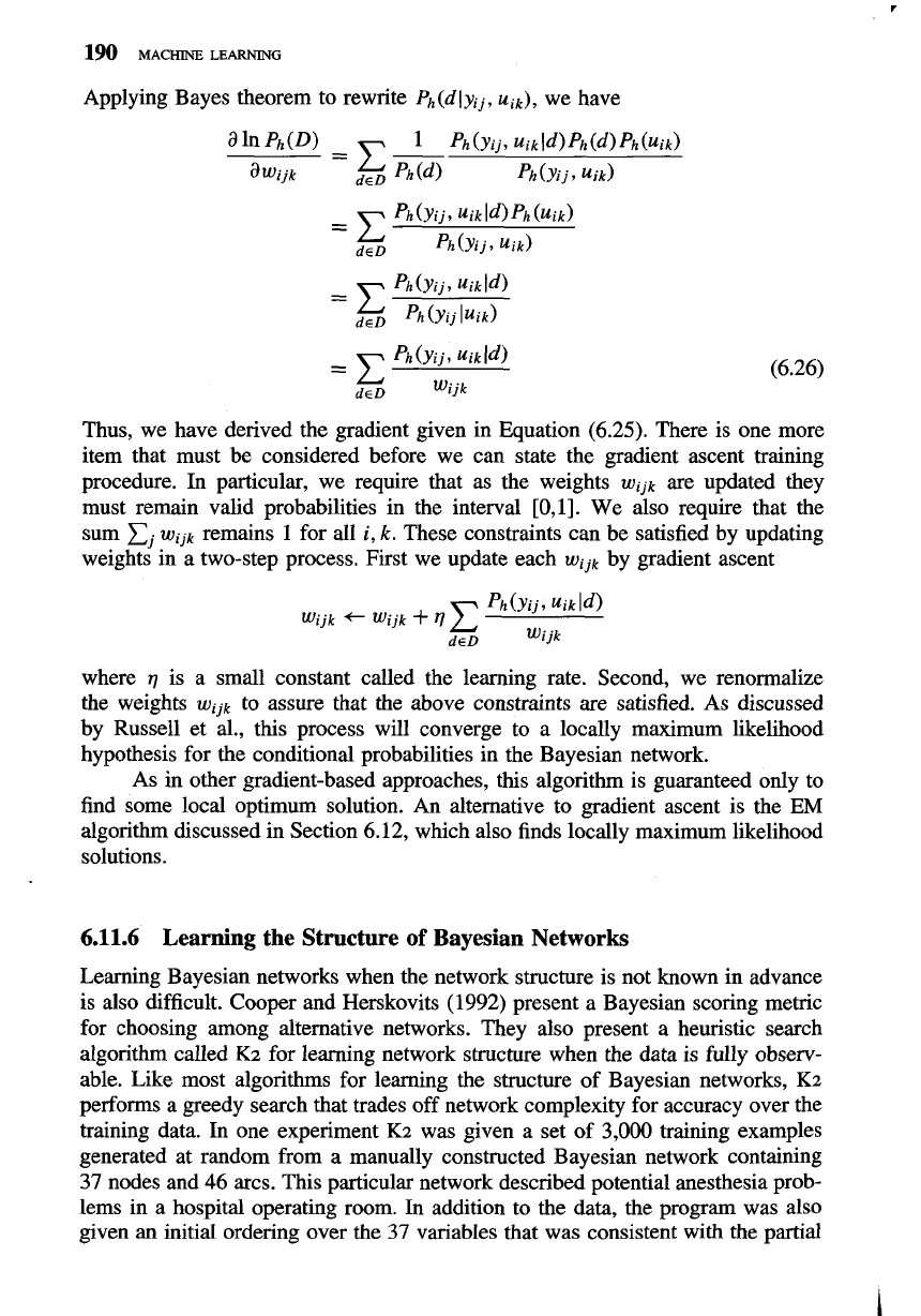
Applying Bayes theorem to rewrite

(dlyij, uik),

we have

Thus, we have derived the gradient given in Equation (6.25). There is one more

item that must be considered before we can state the gradient ascent training

procedure. In particular, we require that as the weights

wijk

are updated they

must remain valid probabilities in the interval [0,1]. We also require that the

sum

wijk

remains 1 for all

These constraints can be satisfied by updating

weights in a two-step process. First we update each

wijk

by gradient ascent

where

is a small constant called the learning rate. Second, we renormalize

the weights

wijk

to assure that the above constraints are satisfied. As discussed

by Russell et al., this process will converge to a locally maximum likelihood

hypothesis for the conditional probabilities in the Bayesian network.

As in other gradient-based approaches, this algorithm is guaranteed only to

find some local optimum solution.

alternative to gradient ascent is the

algorithm discussed in Section 6.12, which also finds locally maximum likelihood

solutions.

6.11.6 Learning the Structure of Bayesian Networks

Learning Bayesian networks when the network structure is not known in advance

is also difficult. Cooper and Herskovits (1992) present a Bayesian scoring metric

for choosing among alternative networks. They also present

heuristic search

algorithm called

for learning network structure when the data is fully observ-

able. Like most algorithms for learning the structure of Bayesian networks,

performs a greedy search that trades off network complexity for accuracy over the

training data. In one experiment

was given a set of 3,000 training examples

generated at random from a manually constructed Bayesian network containing

nodes and 46 arcs. This particular network described potential anesthesia prob-

lems in a hospital operating room. In addition to the data, the program was also

given an initial ordering over

the

37 variables that was consistent with the partial

CHAPTER

BAYESIAN

LEARNING

191

ordering of variable dependencies in the actual network. The program succeeded

in reconstructing the correct Bayesian network structure almost exactly, with the

exception of one incorrectly deleted arc and one incorrectly added arc.

Constraint-based approaches to learning Bayesian network structure have

also been developed

(e.g., Spirtes et al. 1993). These approaches infer indepen-

dence and dependence relationships from the data, and then use these relation-

ships to construct Bayesian networks. Surveys of current approaches to learning

Bayesian networks are provided by Heckerman (1995) and

Buntine (1994).

6.12

THE EM ALGORITHM

In many practical learning settings, only a subset of the relevant instance features

might be observable. For example, in training or using the Bayesian belief network

of Figure 6.3, we might have data where only a subset of the network variables

Storm, Lightning, Thunder, ForestFire, Campfire,

and

BusTourGroup

have been

observed. Many approaches have been proposed to handle the problem of learning

in the presence of unobserved variables. As we saw in Chapter 3, if some variable

is sometimes observed and sometimes not, then we can use the cases for which

it has been observed to learn to predict its values when it is not. In this section

we describe the EM algorithm (Dempster et al. 1977), a widely used approach

to learning in the presence of unobserved variables. The EM algorithm can be

used even for variables whose value is never directly observed, provided the

general form of the probability distribution governing these variables is known.

The EM algorithm has been used to train Bayesian belief networks (see Heckerman

1995) as well as radial basis function networks discussed in Section 8.4. The EM

algorithm is also the basis for many unsupervised clustering algorithms

(e.g.,

Cheeseman et al. 1988), and it is the basis for the widely used Baum-Welch

forward-backward algorithm for learning Partially Observable Markov Models

(Rabiner 1989).

6.12.1

Estimating Means

Gaussians

The easiest way to introduce the EM algorithm is via an example. Consider a

problem in which the data

is a set of instances generated by a probability

distribution that is a mixture of

distinct Normal distributions. This problem

setting is illustrated in Figure 6.4 for the case where

and where the instances

are the points shown along the

axis. Each instance is generated using

two-step

process. First, one of the

Normal distributions is selected at random. Second,

single random instance

is generated according to this selected distribution.

This process is repeated to generate a set of data points as shown in the figure. To

simplify our discussion, we consider the special case where the selection of the

single Normal distribution at each step is based on choosing each with uniform

probability, where each of the

Normal distributions has the same variance

a2,

and

where

is known. The learning task is to output a hypothesis

(FI,

. .

pk)

that describes the means of each of the

distributions. We would like to find

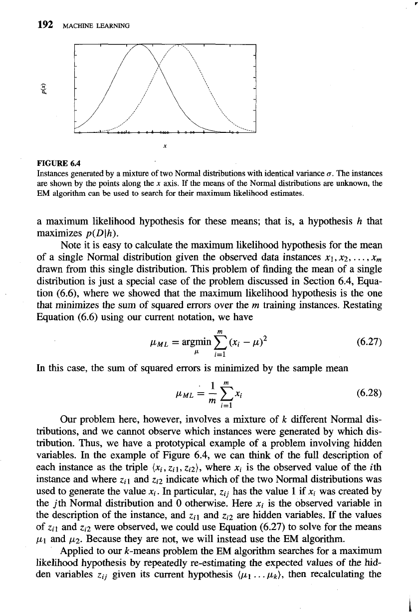
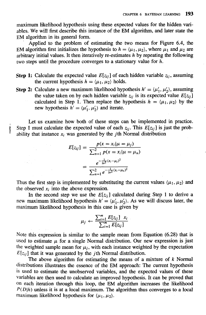
FIGURE

6.4

Instances generated by a mixture of two Normal distributions with identical variance

The instances

are shown by the points along the

axis.

the means of the Normal distributions are unknown, the

algorithm

can

be used to search for their maximum likelihood estimates.

a maximum likelihood hypothesis for these means; that is, a hypothesis h that

maximizes

p(D

lh).

Note it is easy to calculate the maximum likelihood hypothesis for the mean

of a single Normal distribution given the observed data instances

XI,

x2,

. .

drawn from this single distribution. This problem of finding the mean of a single

distribution is just a special case of the problem discussed in Section 6.4, Equa-

tion (6.6), where we showed that the maximum likelihood hypothesis is the one

that minimizes the sum of squared errors over the

training instances. Restating

Equation (6.6) using our current notation, we have

In this case, the sum of squared errors is minimized by the sample mean

Our problem here, however, involves a mixture of k different Normal dis-

tributions, and we cannot observe which instances were generated by which dis-

tribution. Thus, we have a prototypical example of a problem involving hidden

variables. In the example of Figure 6.4, we can think of the full description of

each instance as the triple

(xi,

zil

ziz),

where

is the observed value of the ith

instance and where

zil

and

zi2

indicate which of the two Normal distributions was

used to generate the value

xi.

In particular,

zij

has the value 1 if

was created by

the jth Normal distribution and

otherwise. Here

is the observed variable in

the description of the instance, and

zil

and

zi2

are hidden variables. If the values

zil

and

zi2

were observed, we could use Equation (6.27) to solve for the means

and

p2.

Because they are not, we will instead use the

algorithm.

Applied to our k-means problem the

algorithm searches for a maximum

likelihood hypothesis by repeatedly re-estimating the expected values of the hid-

den variables

zij

given its current hypothesis

(pI

. . .

pk),

then recalculating the

CHAPTER

BAYESIAN

LEARNING

193

maximum likelihood hypothesis using these expected values for the hidden vari-

ables. We will first describe this instance of the EM algorithm, and later state the

algorithm in its general form.

Applied to the problem of estimating the two means for Figure

6.4,

the

algorithm first initializes the hypothesis to

(PI,

p2),

where

and

are

arbitrary initial values. It then iteratively re-estimates

by repeating the following

two steps until the procedure converges to a stationary value for

Step

Calculate the expected value

E[zij]

of each hidden variable

zi,,

assuming

the current hypothesis

(p1, p2)

holds.

Step

Calculate a new maximum likelihood hypothesis

(pi, p;),

assuming

the value taken on by each hidden variable

zij

is its expected value

E[zij]

calculated in Step

Then replace the hypothesis

(pl, p2)

by the

new hypothesis

(pi, pi)

and iterate.

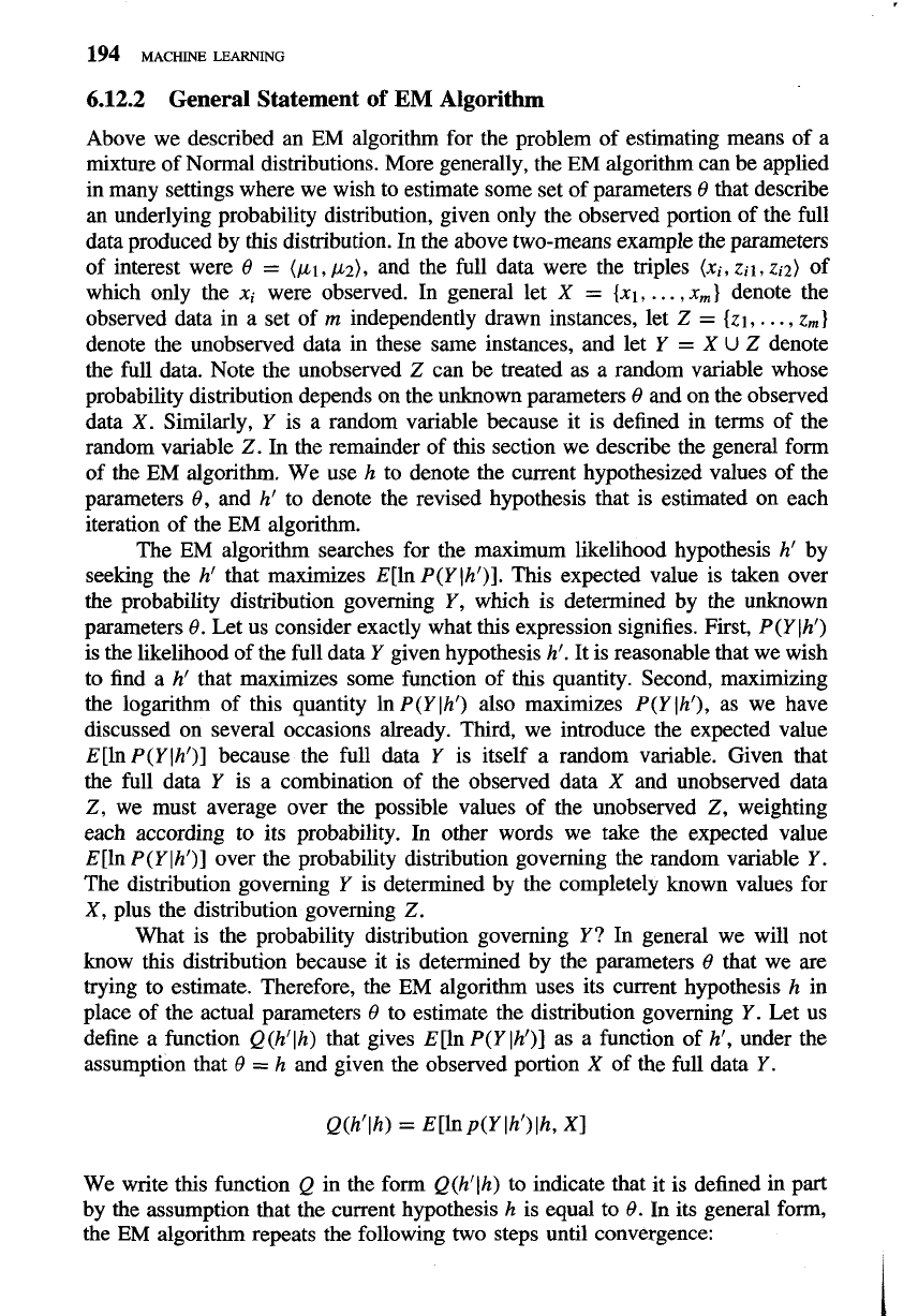
Let us examine how both of these steps can be implemented in practice.

Step

must calculate the expected value of each

zi,.

This

E[4]

is just the prob-

ability that instance

was generated by the jth Normal distribution

Thus the first step is implemented by substituting the current values

(pl, p2)

and

the observed

into the above expression.

In the second step we use the

E[zij]

calculated during Step

to derive a

new maximum likelihood hypothesis

(pi, pi).

AS we will discuss later, the

maximum likelihood hypothesis in this case is given by

Note this expression is similar to the sample mean from Equation

(6.28)

that is

used

to estimate

for a single Normal distribution. Our new expression is just

the weighted sample mean for

pj,

with each instance weighted by the expectation

E[z,j]

that it was generated by the jth Normal distribution.

The above algorithm for estimating the means of a mixture of

Normal

distributions illustrates the essence of the EM approach: The current hypothesis

used to estimate the unobserved variables, and the expected values of these

variables are then used to calculate an improved hypothesis. It can

proved that

on each iteration through this loop, the EM algorithm increases the likelihood

P(Dlh)

unless it is at a local maximum. The algorithm thus converges to a

local

maximum likelihood hypothesis for

(pl,

w2).

6.12.2

General Statement of

Algorithm

Above we described an EM algorithm for the problem of estimating means of a

mixture of Normal distributions. More generally, the EM algorithm can be applied

in many settings where we wish to estimate some set of parameters

that describe

an underlying probability distribution, given only the observed portion of the full

data produced by this distribution. In the above two-means example the parameters

of interest were

(PI, p2),

and the full data were the triples

(xi, zil, zi2)

which only the

were observed. In general let

{xl,

. . .

x,}

denote the

observed data in a set of

independently drawn instances, let

{zl,

. . .

z,}

denote the unobserved data in these same instances, and let

denote

the full data. Note the unobserved

can be treated as a random variable whose

probability distribution depends on the unknown parameters

and on the observed

data

Similarly,

is a random variable because it is defined in terms of the

random variable

In the remainder of this section we describe the general form

of the EM algorithm. We use

to denote the current hypothesized values of the

parameters

and

to denote the revised hypothesis that is estimated on each

iteration of the EM algorithm.

The EM algorithm searches for the maximum likelihood hypothesis

seeking the

that maximizes E[ln

P(Y (h')].

This expected value is taken over

the probability distribution governing

which is determined by the unknown

parameters

Let us consider exactly what this expression signifies. First,

P(Ylhl)

is the likelihood of the full data

given hypothesis

h'.

It is reasonable that we wish

to find a

that maximizes some function of this quantity. Second, maximizing

the logarithm of this quantity In

P(Ylhl)

also maximizes

P(Ylhl),

as we have

discussed on several occasions already. Third, we introduce the expected value

E[ln

P(Ylhl)]

because the full data

is itself a random variable. Given that

the full data

is a combination of the observed data

and unobserved data

we must average over the possible values of the unobserved

weighting

each according to its probability. In other words we take the expected value

E[ln

P(Y lh')]

over the probability distribution governing the random variable

The distribution governing

is determined by the completely known values for

plus the distribution governing

What is the probability distribution governing

In general we will not

know this distribution because it is determined by the parameters

that we are

trying to estimate. Therefore, the EM algorithm uses its current hypothesis

place of the actual parameters

to estimate the distribution governing

Let us

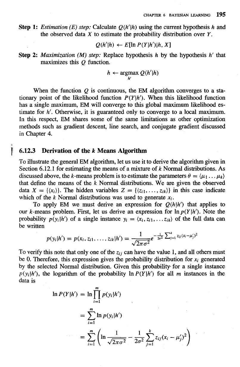
define a function

Q(hllh)

that gives E[ln

P(Y lh')]

as a function of

h',

under the

assumption that

and given the observed portion

of the full data

We write this function

in the form

Q(hllh)

to indicate that it is defined in part

by the assumption that the current hypothesis

is equal to

In its general form,

the

algorithm repeats the following two steps until convergence:

CHAPTER

BAYESIAN

LEARNING

195

Step

Estimation

(E)

step:

Calculate

Q(hllh)

using the current hypothesis

and

the observed data

to estimate the probability distribution over

Q(hf(h)

E[ln

P(Ylhl)lh,

Step

Maximization (M) step:

Replace hypothesis

by the hypothesis

that

maximizes this

function.

argmax

Q (hf

When the function

is continuous, the EM algorithm converges to a sta-

tionary point of the likelihood function

P(Y(hl).

When this likelihood function

has a single maximum, EM will converge to this global maximum likelihood es-

timate for

h'.

Otherwise, it is guaranteed only to converge to a local maximum.

In this respect, EM shares some of the same limitations as other optimization

methods such as gradient descent, line search, and conjugate gradient discussed

Chapter

6.12.3

Derivation of the

Means Algorithm

To illustrate the general EM algorithm, let us use it to derive the algorithm given in

Section

6.12.1

for estimating the means of a mixture of k Normal distributions. As

discussed above, the k-means problem is to estimate the parameters

(PI.

. .

pk)

that define the means of the

Normal distributions. We are given the observed

data

{(xi)}.

The hidden variables

{(zil,

. .

zik)}

in this case indicate

which of the k Normal distributions was used to generate

xi.

To apply EM we must derive an expression for

Q(h(hf)

that applies to

our k-means problem. First, let us derive an expression for

1np(Y(h1).

Note the

probability

p(yi (h')

of a single instance

(xi,

Zil,

. .

~ik)

of the full data can

be written

To verify this note that only one of the

zij

can have the value

and all others must

Therefore, this expression gives the probability distribution for

generated

by the selected Normal distribution. Given this probability for a single instance

p(yi(hl),

the logarithm of the probability In

P(Y(hl)

for all

instances in the

data is

lnP(Ylhf)

lnnp(,lhl)

i=l

Finally we must take the expected value of this In P(Ylhl) over the probability

distribution governing

or, equivalently, over the distribution governing the un-

observed components zij of

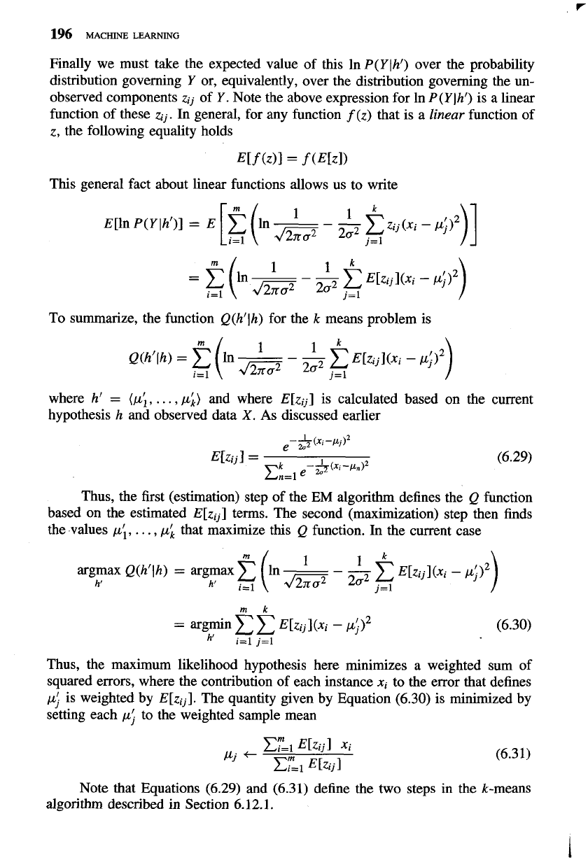
Note the above expression for In P(Ylhl) is a linear

function of these zij. In general, for any function

(z) that is a

linear

function of

z, the following equality holds

E[f (z)l

(Ek.1)

This general fact about linear functions allows us to write

To summarize, the function

Q(hllh) for the k means problem is

where h'

(pi,

. . .

,pi)

and where E[zij] is calculated based on the current

hypothesis h and observed data

As discussed earlier

e-&(x'-~)2

E[zij]

--+

--P")~

(6.29)

EL1

Thus, the first (estimation) step of the

algorithm defines the Q function

based on the estimated E[zij] terms. The second (maximization) step then finds

the values

pi,

. . .

that maximize this Q function. In the current case

argmax Q(hllh)

argmax

E[zijI(xi

i=l

2u2

j=l

Thus, the maximum likelihood hypothesis here minimizes a weighted sum of

squared errors, where the contribution of each instance xi to the error that defines

is weighted by E[zij]. The quantity given by Equation (6.30) is minimized by

setting each

to the weighted sample mean

Note that Equations (6.29) and (6.31) define the two steps in the k-means

algorithm described in Section 6.12.1.

CHAPTER

BAYESIAN

LEARNING

197

6.13

SUMMARY AND FURTHER

READING

The main points of this chapter include:

Bayesian methods provide the basis for probabilistic learning methods that

accommodate (and require) knowledge about the prior probabilities of alter-

native hypotheses and about the probability of observing various data given

the hypothesis. Bayesian methods allow assigning a posterior probability to

each candidate hypothesis, based on these assumed priors and the observed

data.

Bayesian methods can be used to determine the most probable hypothesis

given the data-the maximum a posteriori (MAP) hypothesis. This is the

optimal hypothesis in the sense that no other hypothesis is more likely.

The Bayes optimal classifier combines the predictions of all alternative hy-

potheses, weighted by their posterior probabilities, to calculate the most

probable classification of each new instance.

The naive Bayes classifier is a Bayesian learning method that has been found

useful in many practical applications. It is called "naive" because it in-

corporates the simplifying assumption that attribute values are conditionally

independent, given the classification of the instance. When this assumption

is met, the naive Bayes classifier outputs the MAP classification. Even when

this assumption is not met, as in the case of learning to classify text, the

naive Bayes classifier is often quite effective. Bayesian belief networks pro-

vide a more expressive representation for sets of conditional independence

assumptions among subsets of the attributes.

The framework of Bayesian reasoning can provide a useful basis for ana-

lyzing certain learning methods that do not directly apply Bayes theorem.

For example, under certain conditions it can be shown that minimizing the

squared error when learning a real-valued target function corresponds to

computing the maximum likelihood hypothesis.

The Minimum Description Length principle recommends choosing the hy-

pothesis that minimizes the description length of the hypothesis plus the

description length of the data given the hypothesis. Bayes theorem and ba-

sic results from information theory can be used to provide a rationale for

this principle.

In many practical learning tasks, some of the relevant instance variables

may be unobservable. The

algorithm provides a quite general approach

to learning in the presence of unobservable variables. This algorithm be-

gins with an arbitrary initial hypothesis. It then repeatedly calculates the

expected values of the hidden variables (assuming the current hypothesis

is correct), and then recalculates the maximum likelihood hypothesis (as-

suming the hidden variables have the expected values calculated by the first

step). This procedure converges to a local maximum likelihood hypothesis,

along with estimated values for the hidden variables.

There are many good introductory texts on probability and statistics, such

as Casella and Berger

(1990).

Several quick-reference books (e.g., Maisel

1971;

Speigel

1991)

also provide excellent treatments of the basic notions of probability

and statistics relevant to machine learning.

Many of the basic notions of Bayesian classifiers and least-squared error

classifiers are discussed by Duda and Hart

(1973).

Domingos and Pazzani

(1996)

provide an analysis of conditions under which naive Bayes will output optimal

classifications, even when its independence assumption is violated (the key here

is that there are conditions under which it will output optimal classifications even

when the associated posterior probability estimates are incorrect).

Cestnik

(1990)

provides a discussion of using the m-estimate to estimate

probabilities.

Experimental results comparing various Bayesian approaches to decision tree

learning and other algorithms can be found in Michie et al.

(1994).

Chauvin and

Rumelhart

(1995)

provide a Bayesian analysis of neural network learning based

on the

BACKPROPAGATION

algorithm.

discussion of the Minimum Description Length principle can be found in

Rissanen

(1983, 1989).

Quinlan and Rivest

(1989)

describe its use in avoiding

overfitting in decision trees.

EXERCISES

6.1.

Consider again the example application of Bayes rule in Section 6.2.1. Suppose the

doctor decides to order a second laboratory test for the same patient, and suppose

the second test returns a positive result as well. What are the posterior probabilities

cancer

and

-cancer

following these two tests? Assume that the two tests are

independent.

6.2.

In the example of Section 6.2.1 we computed the posterior probability of cancer by

normalizing the quantities

P (+(cancer)

P (cancer)

and

P (+I-cancer)

P (-cancer)

so that they summed to one, Use Bayes theorem and the theorem of total probability

(see Table 6.1) to prove that this method is valid (i.e., that normalizing in this way

yields the correct value for

P(cancerl+)).

6.3.

Consider the concept learning algorithm

FindG,

which outputs a maximally general

consistent hypothesis (e.g., some maximally general member of the version space).

(a)

Give a distribution for

P(h)

and

P(D1h)

under which

FindG

is guaranteed to

output a MAP hypothesis.

(6)

Give a distribution for

P(h)

and

P(D1h)

under which

FindG

is not guaranteed

to output a MAP .hypothesis.

(c)

Give a distribution for

P(h)

and

P(D1h)

under which

FindG

is guaranteed to

output a

hypothesis but not a MAP hypothesis.

6.4.

In the analysis of concept learning in Section 6.3 we assumed that the sequence of

instances

(xl

. .

x,)

was held fixed. Therefore, in deriving an expression for

P(D(h)

we needed only consider the probability of observing the sequence of target values

(dl.. .dm)

for this fixed instance sequence. Consider the more general setting in

which the instances are not held fixed, but are drawn independently from some

probability distribution defined over the instance space

The data

must now

be described as the set of ordered pairs

{(xi,

di)},

and

P(D1h)

must now reflect the