Middleton W.M. (ed.) Reference Data for Engineers: Radio, Electronics, Computer and Communications
Подождите немного. Документ загружается.

33-30
,’
/
/
/
REFERENCE
DATA
FOR ENGINEERS
-7
-8
-9
-
10
-
l2
3
-
14
5
‘
,,,
graph
Co.)
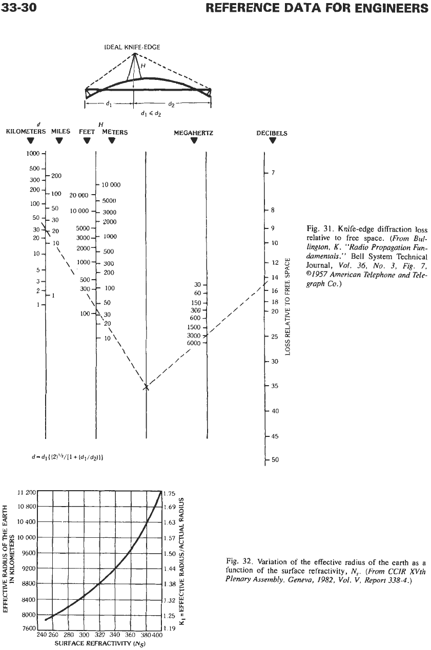
Fig. 31. Knife-edge diffraction
loss
relative to free space.
(From
Bul-
lington,
K.
“Radio Propagation
Fun-
damentuls.”
Bell
System Technical
Journal,
Vol.
36,
No.
3,
Fig.
7,
01957
American Telephone and Tele-
,/-16
5
-18
e
-20
2
9
s
I-
-25
v)
-
30
-
35
-
40
-
45
-
50
IDEAL KNIFE-EDGE
5-
3-
2-
1-
d
H
KILOMETERS MILES FEET METERS
vvv
-1
1000
::~200
200
100
20
000
-
50 10000
-
3000-
\
2000-
10
\\
1000-
\
500
-
300
-
\
\
100-
v
0
000
3000
3000
2000
1000
500
300
200
100
50
30
‘20
\
10
\
\
\
\
\
\
v
30.
60.
150.
300
’
600.
1500
3000
6000
/
/
/
/
/
MEGAHERTZ DECIBELS
v
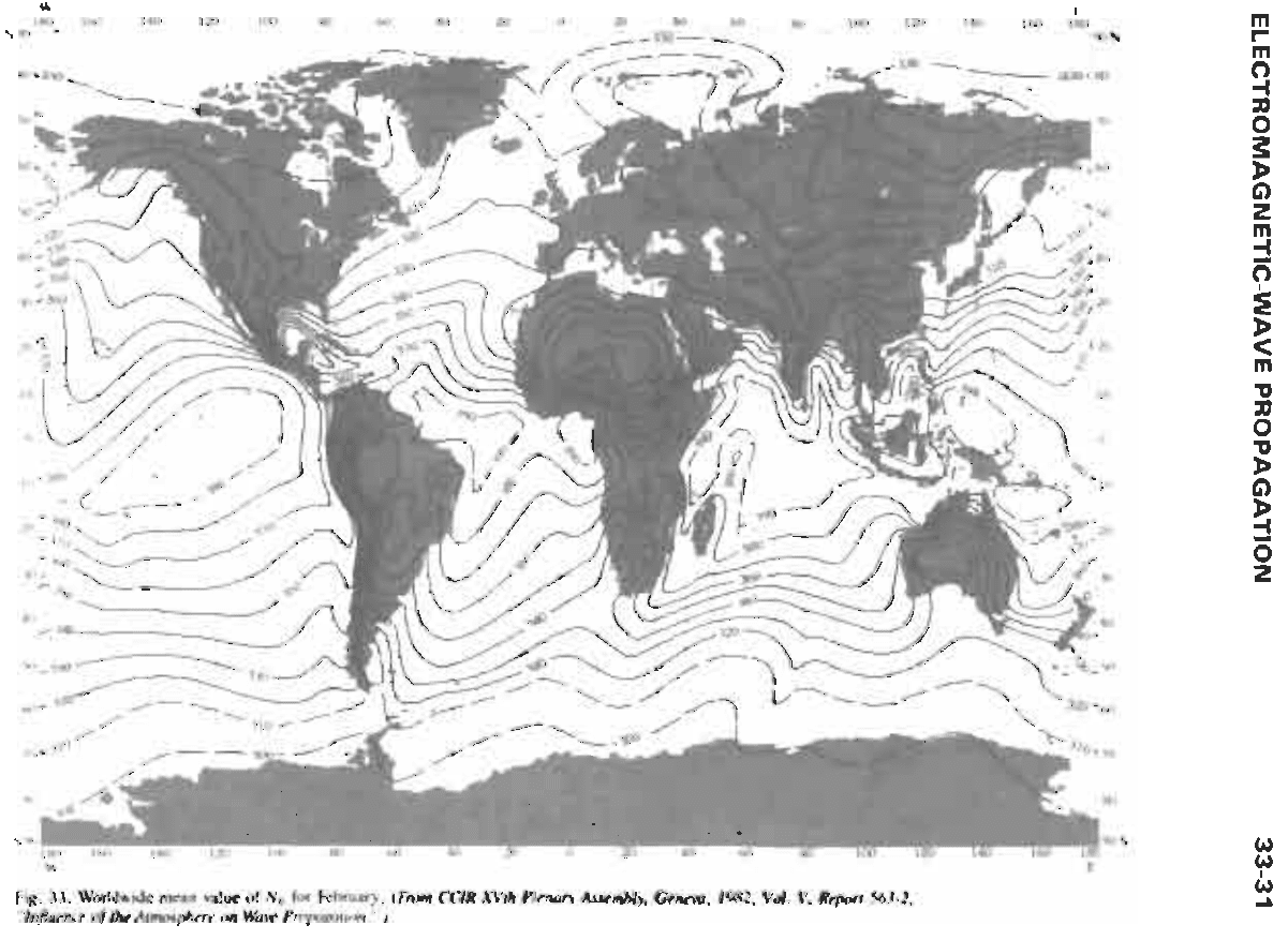
Fig.
32.
Variation
of
the effective radius
of
the earth as a
function
of
the surface refractivity,
N,.
(From CCIR XVth
Plenary Assembly, Geneva,
1982,
Vol.
V,
Report
338-4.)
SCJRFACE REFRACTIVITY
(Ns)
ELECTROMAGNETIC-WAVE PROPAGATION
33-3
1
33-32
REFERENCE
DATA
FOR ENGINEERS
Od
Fig.
34.
Attenuation function
F(Bd),
where
d
is in kilometers
and
0
is
in radians, for indicated values of surface refractivity
N,.
(From CCIR XVth Plenary Assembly, Geneva, 1982,
Vol.
V,
Report 238-4.)
of
60
wavelengths usually being adequate. Slow fading,
with periods of hours or days, is caused by changes in
the gradient of the refractive index of the atmosphere
along the transmission path and is little affected by
diversity.
The plane-wave gains
of
large antennas are not fully
realized
on tropospheric scatter paths. The power
on
de
IN
KILOMETERS
1.
2.
Continental subtropical (Sudan)
3
4. Desert (Sahara)
5.
Mediterranean
(no
curves available)
6
ia. Maritime temperate.
over
land
(data from U.K
I
7b. Maritime temperate,
over
sea
(data from
U.K
j
8.
Polar
(no
curves
available)
Equatorial (data from Congo and Ivory
Coast)
Maritime subtropical (data from West
Coast
of Africa)
Continental tempmate (data
from
France.
Federal Republic
of
Germany.
and
U.5
A
i
Fig.
35.
Function
V(d,)
for the types of climate indicated
on
the curves.
(From CCIR
XVth
Plenary Assembly, Geneva,
1982,
Vol.
V,
Report 2384.)
such a path is received, not from a single point source,
but from a volume in the atmosphere that subtends a
solid angle at the receiving antenna. If the antenna
beam angles are such as to limit the available scattering
volume, then the received power will be corresponding-
ly limited, and the antennas are said to suffer an
antenna-to-medium coupling loss. The resulting medi-
an loss of received power is likely to be about
5
decibels
for two 40-decibel-gain plane-wave antennas, and
17
decibels for two 50-decibel-gain antennas. The extent
to
which the path antenna gain is a function of the scatter
angle,
8,
or the height of the scatter volume has not yet
been established.
Multipath transmission limits the communication
bandwidth that can be used
on
a single carrier; however,
useful bandwidths of several megahertz have been
shown to be available
on
some 200-mile scatter paths.
Narrow-beam antennas and diversity reduce the effects
of multipath transmission.
u
w
P
5
Y
7
$
5
:
A
B
C
D
E
F
G
H
J
K
L
M
IC_
MEGAHERTZ
+-
GIGAHERTZ
4
FREQUENCY
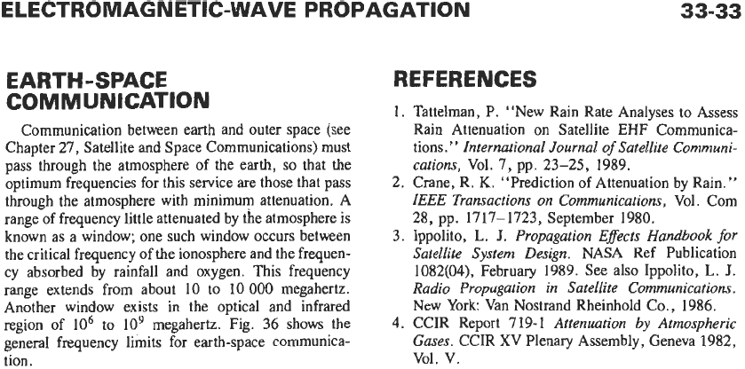
Signal lewel during ideal nighttime conditions
(no
absorption)
Typical signal level
during
daytime conditions. assuming an
angle
of ele-
Minimum frequency to assure penetration
of
ionosphere polar
region.
Minimum frequency
to
assure
penetration of ionosphere: tropical
region.
Beam width of paraboloid between half-power points.
Effect of ionospheric absorption.
Minimum cosmic noise Maximum
value
will be found
to
be higher by
about
15
decibels.
Noise level corresponding
to
a
temperature of
70
kelvins
Noise due to absorption
in
a
clear
atmosphere. assuming
an
elevation
Typical signal level for
a
vertical path
~n
a
clear
atmosphere
Typical signal level in heavy rain
(16
millimeters/hour), vertical depth
1
Effect of varying atmospheric conditions and elevation angles.
vation of
5O
oblique path: tropical region, vertical path
oblique path
angle
of
5O
kilometer, assuming an elevation angle of
5%
Fig.
36.
General frequency limits in
a
simple earth-to-
spacecraft communication system. (Spacecraft: isotropic an-
tenna; transmitter power,
1
watt; bandwidth,
1
kilohertz;
distance,
1000
kilometers. Earth station antenna: paraboloid;
diameter,
20
meters; efficiency,
55%--.
15-decibel gain
above isotropic antenna
- -
-.)
(From CCIR Xth Plenary
Assembly, Geneva, 1963,
Vol.
IV,
Report 205,
p.
194.)
ELECTROMAGNETIC-WAVE PROPAGATION
EARTH-SPACE
COMMUNICATION
Communication between earth and outer space (see
Chapter 27, Satellite and Space Communications) must
pass through the atmosphere of the earth,
so
that the
optimum frequencies for this service
are
those that pass
through the atmosphere with minimum attenuation. A
range of frequency little attenuated by the atmosphere is
known as a window; one such window occurs between
the critical frequency of the ionosphere and the frequen-
cy absorbed by rainfall and oxygen. This frequency
range extends from about 10 to
10
000
megahertz.
Another window exists in the optical and infrared
region of
lo6
to
lo9
megahertz. Fig.
36
shows the
general frequency limits for earth-space communica-
tion.
REFERENCES
33-33
1. Tattelman, P. “New Rain Rate Analyses to Assess
Rain Attenuation
on
Satellite
EHF
Communica-
tions.
’
International Journal
of
Satellite Communi-
cations,
Vol. 7, pp. 23-25, 1989.
2. Crane, R.
K.
“Prediction of Attenuation by Rain.”
IEEE Transactions
on
Communications,
Vol
.
Corn
28, pp. 1717-1723, September 1980.
3. Ippolito,
L.
J.
Propagation Effects Handbook for
Satellite System Design.
NASA Ref Publication
1082(04), February 1989. See also Ippolito,
L.
J.
Radio Propagation in Satellite Communications.
New York: Van Nostrand Rheinhold Co., 1986.
4. CCIR Report 719-1
Attenuation by Atmospheric
Gases.
CCIR XV Plenary Assembly, Geneva 1982,
VOl.
v.
34
Radio Noise and
Interference
Revised
by
George
W.
Swenson,
Jr. and
A.
Richard Thompson
Natural Noise
34-2
Thermal Noise
Atmospheric Noise
Cosmic Noise
Man-Made Radio Noise
34-6
Near-Zone and Far-Zone Noise Sources
Power Line Noise
Precipitation Static
34-8
Thermal Noise Calculations
34-8
Noise Measurements
34-8
Measurement for Broadcast Receivers
Noise Factor
of
a Receiver
Measurement of Noise Figure With a Thermal Noise Source
Calculation of Noise Figure
Noise Factor
of
Cascaded Networks
Interference From Signals
of
Other Services
34-11
34-
1
34-2
REFERENCE
DATA
FOR
ENGINEERS
Radio noise and interference limit the performance of
all communications systems by restricting the operating
range, generating errors in messages, and in extreme
cases preventing the successful operation of receivers.
At
locations where man-made noise is low, natural
noise sources determine receiver performance. When
man-made noise encroaches upon receiving sites, the
performance of receiving equipment is degraded below
design levels.
When noise from sources external to a receiver is
involved, the gain and orientation of the antenna must
be considered. For narrow-band receivers, noise is
usually flat in amplitude across the bandwidth of a
receiver. For such cases, noise power affecting receiver
performance is proportional to the bandwidth. For
wideband receivers, the noise may not be flat across the
receiver bandwidth, and the determination of effective
noise power requires further consideration.
Noise level can be expressed in terms of voltage or
power
at
the terminals of a receiver, the strength of an
electromagnetic field at an antenna location, or thermal
noise power at a temperature referenced to
290
kelvins.
Noise that is flat in amplitude across the bandwidth of a
receiver is often expressed in terms of an effective
antenna noise factor,-&, which is defined
f,
=
P,,/kToB
=
T,/To
where,
as
0%.
1)
P,,
=
noise power in watts from an equivalent
lossless antenna,
k
=
Boltzmann’s constant,
To
=
reference temperature
(290
kelvins),
B
=
receiver noise bandwidth in hertz,
T,
=
antenna noise temperature in the presence of
external noise.
NATURAL NOISE
Natural noise consists of thermal noise, atmospheric
noise, and cosmic noise. These noise sources usually
FREQUENCY
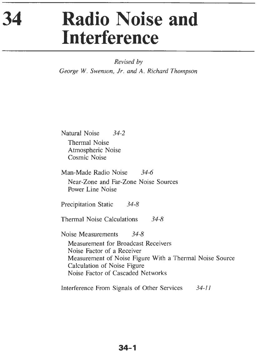
Fig.
1.
Noise figure
(F)
and noise temperature
(T,)
for various devices and natural limits--1984.
(From
S.
Weinreb, “Low-Noise
GASFET Amplifiers.”
IEEE Trans.
on
MTT,
Vol.
MTT-28, No.
10,
October 1980, pp. 1041-1054. Material updated to 1984 by
Weinreb
.
)

RADIO NOISE AND INTERFERENCE
34-3
EAST WEST WEST EAST
60°
90"
120°
150°
180°
150°
120"
90O
60°
3Q0
04
30°
6O0
900
900
z
z
30"
30°
EQUATOR
00
T
900
-
(
1
I/
EAST
WEST WEST EAST
Fig.
2.
Atmospheric noise levels in northern
and
southern hemispheres, summer,
1200-1600
hours local time. The maps show the
expected values
of
Fa
at
I
MHz,
in decibels above
kT,B.
(From
CCIR Repon
322,
10th
Plenary
Assemh/y,
Geneva;
1963.)
determine the minimum detectable signal level of a
receiver operated in an environment free of man-made
noise sources.
Themal Noise
For many
years,
thermal noise in the first stage of a
receiver was usually the main factor limiting the sensi-
tivity of radar and microwave receivers. Recent advanc-
es
in low-noise amplifier performance have reduced
thermal noise of microwave amplifiers to very
low
levels, and thermal radiation from nearby objects,
ground, and the sky are now major factors that must
be
considwed in choosing sites for satellite receivers and
radars. Fig.
1
shows noise temperatures for various
devices (as of
1984)
and natural limits at microwave
frequencies. Receivers operated at frequencies below
about
20
MHz
usually encounter noise from other
sources that is considerably above the thermal noise
of
conventional amplifiers; hence, low-noise amplifier
performance
is
not usually a factor in the design of
low-frequency receivers. An exception occurs for
VLF
receivers operating in the Arctic and Antarctic, where
atmospheric noise is extremely low and cosmic noise is
screened by the ionosphere.
Atmospheric Noise
Lightning from thunderstorms produces bursts of
impulsive noise. At low frequencies, these bursts are
propagated to distant receivers by normal ionospheric
modes. The noise is dependent
on
the weather, time of
day, season, location
of
the receiver with respect to
storm areas, and ionospheric propagation conditions.
Atmospheric noise generally decreases with increasing
latitude and increases in high-latitude equatorial areas.
Atmospheric noise sources
are
particularly active dur-
ing the rainy season in the Caribbean, the East Indies,
equatorial Africa, northern India, and the Far East. An
excellent summary of worldwide atmospheric noise
levels is contained in CCIR Report
322.*
An example
of
a CCIR developed map of atmospheric noise levels in
the summer during daytime hours is shown in Fig.
2.
*
CClR
Report
322,
Vol.
VI,
10th Plenary Assembly,
-
Geneva;
1963.
34-4
REFERENCE
DATA
FOR ENGINEERS
x
MAN-MADE
N
z
(QUIET
LOCA-
20
IL'
~~
0
0
01
1
01
10
c!
I
10
7-
f
T
i.
10(
FREQUENCY
IN
MEGAHERTZ
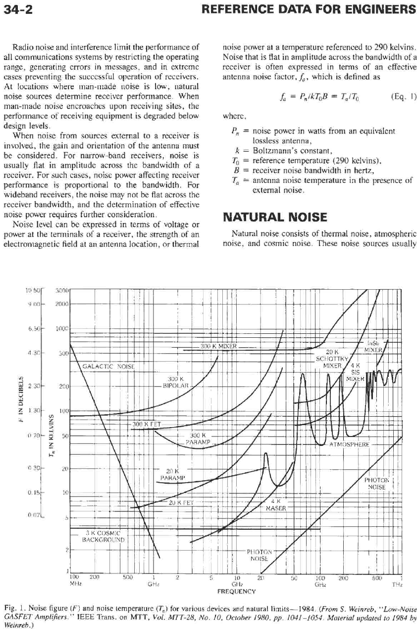
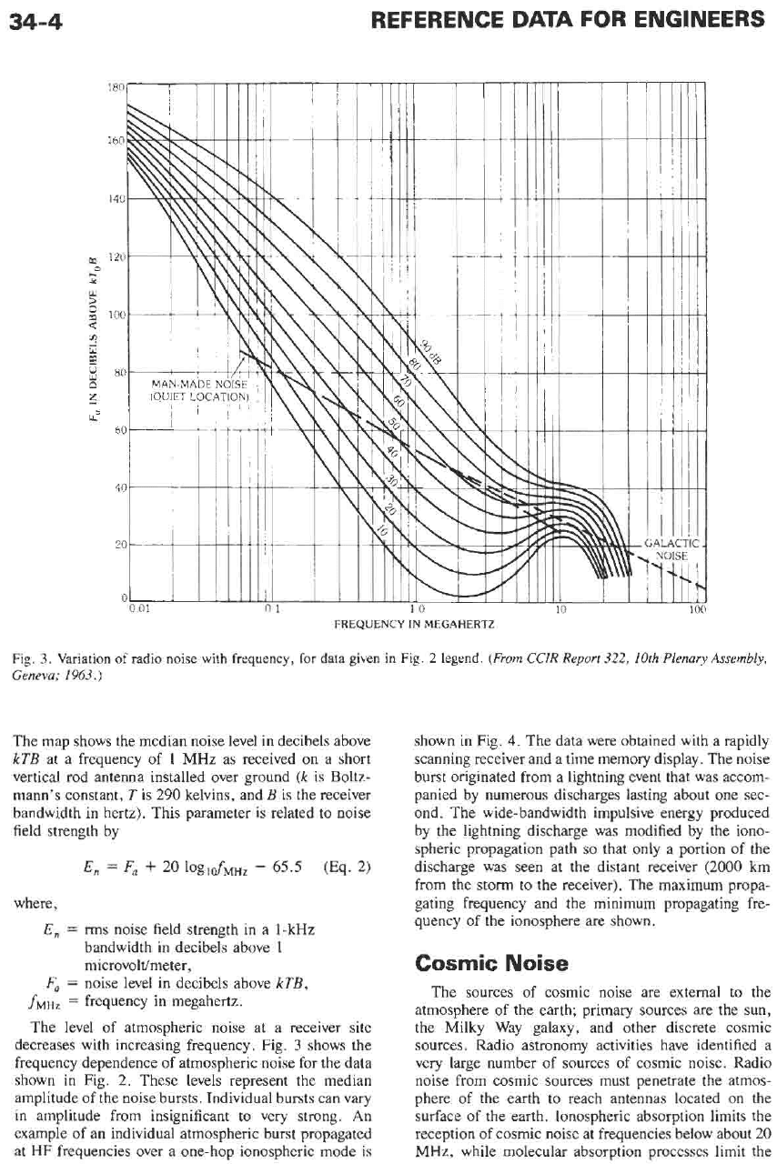
Fig.
3.
Variation
of
radio noise with
frequency,
for
data given
in
Fig.
2
legend.
(From
CUR
Report
322,
10th
Plenary
Assembly,
Geneva;
1963.)
The map shows the median noise level in decibels above
kTB
at a frequency of 1 MHz as received
on
a short
vertical rod antenna installed over ground
(k
is Boltz-
mann's constant,
T
is
290
kelvins, and
B
is the receiver
bandwidth in hertz). This parameter is related
to
noise
field strength by
where,
E,
=
rms
noise field strength in a 1-kHz
bandwidth in decibels above 1
microvolt/meter,
fMHz
=
frequency in megahertz.
The level of atmospheric noise at a receiver site
decreases with increasing frequency. Fig.
3
shows the
frequency dependence of atmospheric noise for the data
shown in Fig.
2.
These levels represent the median
amplitude of the noise bursts. Individual bursts can vary
in amplitude from insignificant to very strong.
An
example of an individual atmospheric burst propagated
at
HF
frequencies over a one-hop ionospheric mode is
Fa
=
noise level in decibels above
RTB,
shown
in
Fig.
4.
The data were obtained with a rapidly
scanning receiver and a time memory display. The noise
burst originated from a lightning event that was accom-
panied by numerous discharges lasting about one sec-
ond. The wide-bandwidth impulsive energy produced
by the lightning discharge was modified by the iono-
spheric propagation path
so
that only a portion of the
discharge was seen at the distant receiver
(2000
km
from the storm to the receiver). The maximum propa-
gating frequency and the minimum propagating fre-
quency of the ionosphere are shown.
Cosmic
Noise
The sources of cosmic noise are external to the
atmosphere of the earth; primary sources are the sun,
the Milky Way galaxy, and other discrete cosmic
sources. Radio astronomy activities have identified a
very large number of sources
of
cosmic noise. Radio
noise from cosmic sources must penetrate the atmos-
phere of the earth to reach antennas located
on the
surface of the earth. Ionospheric absorption limits the
reception of cosmic noise at frequencies below about
20
MHz,
while molecular absorption processes limit the

RADIO NOISE
AND
INTERFERENCE
34-5
1
5
6
5
FREQUENCY IN
MEGAHERTZ
Fig.
4.
Atmospheric noise burst.
reception of extraterrestrial noise at frequencies above
about
10
GHz.
Satellite-borne receivers above about
IO00
km do not encounter these limitations.
Recent advances in low-noise receiver design (see
Fig.
1)
and the widespread deployment of satellites and
space probes have increased the importance of cosmic
noise. Satellite communications systems, the broadcast-
ing of television from satellites, and the need for data
links between the space vehicles and the earth have
increased the number of skyward-pointed antennas
equipped with sensitive receivers that are capable of
receiving cosmic noise. Cosmic noise often limits the
performance of such systems.
Figs.
8
and
9
of Chapter 32 show detailed radio-sky
maps of the celestial sphere for the 136-megahertz and
400-megahertz space research satellite frequency bands.
Fig.
5
shows the level of galactic noise in decibels
relative to a noise temperature of
290
K
when receiving
on a half-wave dipole. The noise levels shown in this
figure assume no atmospheric absorption and refer to
the following sources of cosmic noise.
Galactic
Plane:
Galactic noise from the galactic
plane in the direction of the center of the galaxy. The
noise levels from other parts of the galactic plane can
be
as much as
12
to
IS
decibels below the levels given
in Fig.
5.
Quiet
Sun:
Noise from the “quiet” sun; that is,
solar
noise at times when there is little
or
no sunspot
activity.
Disturbed
Sun:
Noise
from
the “disturbed” sun.
The term “disturbed” refers to times of sunspot and
solar-flare activity.
Cussiopeiu
A:
Noise from a high-intensity discrete
source of cosmic noise known as Cassiopeia
A.
This
is one of thousands of known discrete sources.
Cassiopeia
A
subtends a solid angle at the surface of
the earth of only about
5
arc
minutes.
The levels of cosmic noise received by a highly
directive antenna with main lobe pointed along the
galactic plane can
be
obtained from equations given by
Kraus*
for the antenna-noise temperature
(TA)
at the
output terminals of an ideal, loss-free, antenna as
e=w-eo
6=2~
I, I,
T(ww(e.4)
sin~~4
TA
=
K
c*’”
G(O,4)sineded4
where,
e
=
0”
at zenith,
=
360”
azimuth angle,
T(
($4)
=
brightness-noise temperature. distribution
from radio-sky map, kelvins,
G(8,4)
=
antenna radiation pattern gain
distribution, assumed symmetrical,
antenna main-lobe axis and the horizon,
degrees.
However, for a practical antenna, Taylor and
Stocklint give a simplified approximation for
TA
includ-
ing contributions from the main lobe, side lobes, and
back
lobe
as
0,
=
minimum elevation angle betwen
TA
^I
0.82
qb
+
0.13(FJ1,
+
TE)
K,
for a solid-
angle beam,
OHpB,
=
4HpeW
5
25”
where,
TE
T&
=
mean value of sky-brightness
-
in kelvins,
TSb
=
mean value of sky-brightness
temperature within main-lobe
HPBW,
temperature within antenna side lobes,
in kelvins,
earth.
II=
To
=
290
K,
effective noise temperature of
For example, a 136-megahertz, phased-array, direc-
tive antenna with main-lobe
HPBW
equal to
12”,
pointed near Cassiopeia
A,
has a value of
TA
equalto
approximately
870
K,
for
ch
equal to
950
K
and
T,,
equal to
400
K
obtained from Fig.
8
of Chapter
32.
-
*
J.
D. Kraus,
Radio Astronomy.
New
York: McGraw-Hill
Book
Co.,
1966;
2nd ed.,
Powell,
OH: Cygnus-Quasar
Books,
1986.
t
R.
F. Taylor
and
F.
J.
Stocklin, “VHFNHF Stellar
Calibration
Error
Analysis,”
Proceedings International Tele-
metering Conference,
Washington, D.C., Vol. V11, pp.
553-
566;
September
27-29, 1971.