Menke W. Geophysical Data Analysis: Discrete Inverse Theory
Подождите немного. Документ загружается.


28
2
Some Comments
on
Probability
Theory
r
v
n
d,
0
1
L
0
1
di
0
1
2
dl+d2
Fig.
2.9.
(a and b) The uncorrelated data d, and
d,
both have white distributions on the
interval
[0,
I].
(c) Their joint distribution consists
of
a rectangular area
of
uniform
probability. The probability distribution
for
the
sum
d,
+
d,
is
the joint distribution,
integrated along lines of constant
d,
+
d,
(dashed). (d) The distribution for
d,
+
d2
is
triangular.
Performing this line integral
in
the most general case can be mathe-
matically quite difficult. Fortunately, in the case of the linear function
m
=
Md
+
v,
where M and
v
are an arbitrary matrix and vector,
respectively,
it
is
possible to make some statements about the proper-
ties of the resultant distribution without explicitly performing the
integration. In particular, the mean and covariance of the resultant
distribution can be shown, respectively, to be
(m)
=
M(d)
+
v
and [cov
m]
=
M[cov d]MT
(2.7)
As
an example, consider a model parameter
rn,
,
which
is
the mean
of a set of data
N
rn,
=
l/N~di=(l/N)[l,
1,
I,
.
.
.
,
l]d
(2.8)
i-
I
That
is, M
=
[
1,
1, 1,
.
.
.
,
1
]/Nand
v
=
0.
Suppose that the data are
uncorrelated and all have the same mean
(d)
and variance
0:.
Then

2.4
Gaussian Distributions
29
we see that
(m,)
=
M(d)
+
v
=
(d)
and var(m,)
=
M[cov
d]MT
=
a:/N.
The model parameter
rn,
,
therefore, has a distribution
P(ml)
with mean
(m,
)
=
(d)
and a variance
a’,
=
a:/N.
The square root of
the variance, which is a measure
of
the width of the peak in
P(m,)
and
therefore a measure of the likelihood that any particular experiment
will yield an
m,
close to the true mean, is proportional to
N-1/2.
The
accuracy of determining the mean of a group of data, therefore,
decreases very slowly as the number of observations increases.
2.4
Gaussian Distributions
The distribution for a particular random variable can be an arbi-
trarily complicated function, but in many instances data possess the
rather simple Gaussian distribution
This distribution has mean
(d)
and variance
uz
(Fig.
2.10).
The
Gaussian distribution is
so
common because it is the limiting distribu-
tion for the sum of random variables. The
central
limit
theorem
shows
(with certain limitations) that regardless of the distribution of a set of
independent random variables, the distribution of their sum tends to a
Gaussian distribution as the number of summed variables increases.
As
long as the noise in the data comes from several sources of
comparable size,
it
will tend to follow a Gaussian distribution. This
0.50
-
n
7J
-
0.25
a
-
0
-5
-4
-3
-2
-1
0
1
2
3
4
5
d
Fig.
2.10.
Gaussian distribution with zero mean and
u
=
I
for
curve
A,
and
u
=
2
for
curve
B.

30
2
Some Comments
on
Probability
Theory
behavior is exemplified by the sum of the two white distributions in
Section 2.3. The distribution of their sum is more nearly Gaussian
than the individual distributions (it being triangular instead of rectan-
gular).
The joint distribution for two independent Gaussian variables is just
the product of two univariate distributions. When the data are corre-
lated (say, with mean (d) and covariance [cov d]), the distribution is
more complicated, since it must express the degree of correlation. The
appropriate generalization turns out to be
exp(-i[d
-
(d)lT[cov d]-'[d
-
(d)]
I
[cov d]
(27p
P(d)
=
This distribution is chosen because it has the correct mean and
variance when the data are uncorrelated and has covariance [cov d]
when the data are correlated. It can be shown that all linear functions
of
Gaussian random variables are also Gaussian random variables
with a distribution of this form.
The idea that the model and data are related by an explicit relation-
ship g(m)
=
d can be reinterpreted in light of this probabilistic descrip-
tion of the data. We can no longer assert that this relationship can hold
for the data themselves, since they are random variables. Instead, we
assert that this relationship holds for the mean data: g(m)
=
(d). The
distribution for the data can then be written as
~[COV
dj1-'/2
1
exp
[
-7
[d
-
g(m)lT[cov d]-'[d
-
g(m)]] (2.1
1)
(27p
P(d)
=
The model parameters now have the interpretation of a set of un-
known quantities that define the shape of the distribution for the data.
One approach to inverse theory (which will be pursued in Chapter
5)
is
to try to use the data to determine the distribution, and thus the values
of the model parameters.
For
the Gaussian distribution [Eq. (2.1 l)] to be sensible, g(m) must
not be a function
of
any random variables. This is why we differen-
tiated between data and auxi!iary variables in Chapter
1;
the latter
must be known exactly. If the auxiliary variables are themselves
uncertain, then they must be treated as data and the inverse problem
becomes an implicit one with a much more complicated distribution
than the above problem exhibits.
As
an example of constructing the distribution for a set of data,
consider an experiment in which the temperature
di
in some small
2.5
Testing the Assumption
of
Gaussian Statistics
31
volume of space is measured
N
times. If the temperature is assumed
not to be a function
of
time and space, the experiment can
be
viewed as
the measurement of
N
realizations of the same random variable or as
the measurement of one realization of
N
distinct random variables
that all have the same distribution. We adopt the second viewpoint.
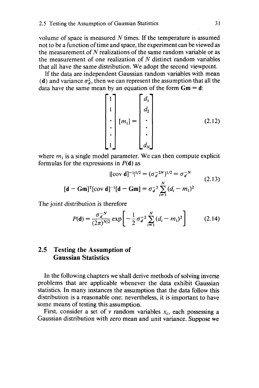
If the data are independent Gaussian random variables with mean
(d)
and variance
03,
then we can represent the assumption that all the
data have the same mean by an equation of the form
Gm
=
d:
[mil
=
(2.12)
where
m,
is a single model parameter. We can then compute explicit
formulas for the expressions in
P(d)
as
[d
-
Gm]*[cov d]-'[d
-
Gm]
=
ai2
C
(di
-
ml)2
i-
1
The joint distribution is therefore
P(d)
=
~
a;N
exp[--a;2x(di-
lN
mJ2]
(2.14)
(27p2 2
i-1
2.5
Testing the Assumption
of
Gaussian Statistics
In the following chapters we shall derive methods of solving inverse
problems that are applicable whenever the data exhibit Gaussian
statistics. In many instances the assumption that the data follow this
distribution is a reasonable one; nevertheless, it is important to have
some means of testing this assumption.
First, consider a set of
v
random variables
xi,
each possessing a
Gaussian distribution with zero mean and unit variance. Suppose we
32
2
Some Comments
on
Probability
Theory
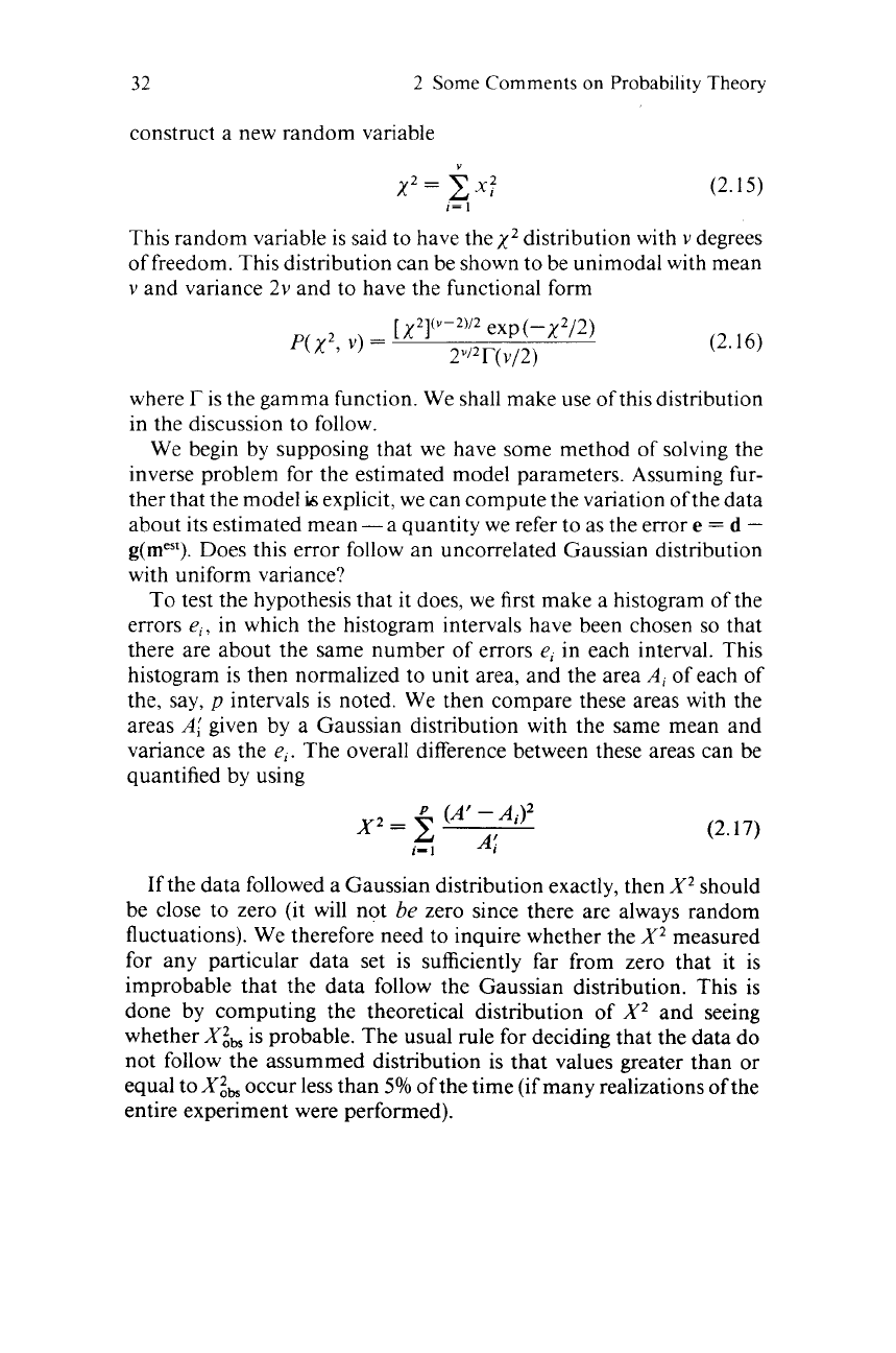
construct a new random variable
(2.15)
This random variable is said to have thex2 distribution with
v
degrees
of freedom. This distribution can be shown to be unimodal with mean
v
and variance 2v and to have the functional form
(2.16)
where is the gamma function. We shall make use of this distribution
in the discussion to follow.
We begin by supposing that we have some method of solving the
inverse problem for the estimated model parameters. Assuming fur-
ther that the model
is
explicit, we can compute the variation ofthe data
about its estimated mean
-
a quantity we refer to as the error
e
=
d
-
g(mest).
Does this error follow an uncorrelated Gaussian distribution
with uniform variance?
To
test the hypothesis that it does, we first make a histogram of the
errors
e,,
in which the histogram intervals have been chosen
so
that
there are about the same number of errors
e,
in each interval. This
histogram is then normalized to unit area, and the area
A,
of each of
the, say,
p
intervals is noted. We then compare these areas with the
areas
Al
given by a Gaussian distribution with the same mean and
variance as the
e,.
The overall difference between these areas can be
quantified by using
P
(A’
-
Ai)2
X2’C
i-
1
A;
(2.17)
If
the data followed a Gaussian distribution exactly, then
X2
should
be close to zero (it will not
be
zero since there are always random
fluctuations). We therefore need to inquire whether the
X2
measured
for any particular data set is sufficiently far from zero that it is
improbable that the data follow the Gaussian distribution. This is
done by computing the theoretical distribution of
X2
and seeing
whether
Xg
is probable. The usual rule for deciding that the data do
not follow the assummed distribution is that values greater than
or
equal to
X&
occur less than
5%
of the time (if many realizations
of
the
entire experiment were performed).
2.6
Confidence Intervals
33
The quantity
X2
can be shown to follow approximately a
x2
distri-
bution, regardless of the type of distribution involved. This method
can therefore be used to test whether the data follow any given
distribution. The number ofdegrees
of
freedom is given byp minus the
number of constraints placed on the observations. One constraint is
that the total area
C
A,
is unity. Two more constraints come from the
fact that we assumed a Gaussian distribution and then estimated the
mean and variance from the
el.
The Gaussian case, therefore, has
v
=
p
-
3.
This test is known as the
x2
test.
The
x2
distribution is
tabulated in most texts on statistics.
2.6
Confidence
Intervals
The confidence of a particular observation is the probability that
one realization of the random variable falls within a specified distance
of the true mean. Confidence is therefore related to the distribution of
area in
P(d).
If
most ofthe area is concentrated near the mean, then the
interval for, say,
95%
confidence will be very small; otherwise, the
confidence interval will be large. The width of the confidence interval
is related to the variance. Distributions with large variances will also
tend to have large confidence intervals. Nevertheless, the relationship
is not direct, since variance is a measure
of
width, not area. The
relationship is easy to quantify for the simplist univariate distribu-
tions.
For
instance, Gaussian distributions have
68%
confidence inter-
vals
la
wide and
95%
confidence intervals
20
wide. Other types of
simple distributions have similar relationships.
If
one knows that a
particular Gaussian random variable has
a
=
1,
then if a realization of
that variable has the value
50,
one can state that there is a
95%
chance
that the mean of the random variable lies between
48
and
52
(one
might symbolize this
by
(d)
=
50
f
2).
The concept of confidence intervals is more difficult to work with
when one is dealing with several correlated data. One must define
some volume in the space of data and compute the probability that the
true means of the data are within the volume. One must also specify
the shape of that volume. The more complicated the distribution, the
more difficult it is to chose an appropriate shape and calculate the
probability within it.
This page intentionally left blank
3
SOLUTION
OF
THE
LINEAR, GAUSSIAN
INVERSE PROBLEM,
VIEWPOINT
1:
THE
LENGTH METHOD
3.1
The Lengths
of
Estimates
The simplest of methods for solving the linear inverse problem
Gm
=
d
is based on measures of the size, or length,
of
the estimated
model parameters
mest
and
of
the predicted data
dPR
=
Gmest.
To
see that measures
of
length can
be
relevant to the solution of
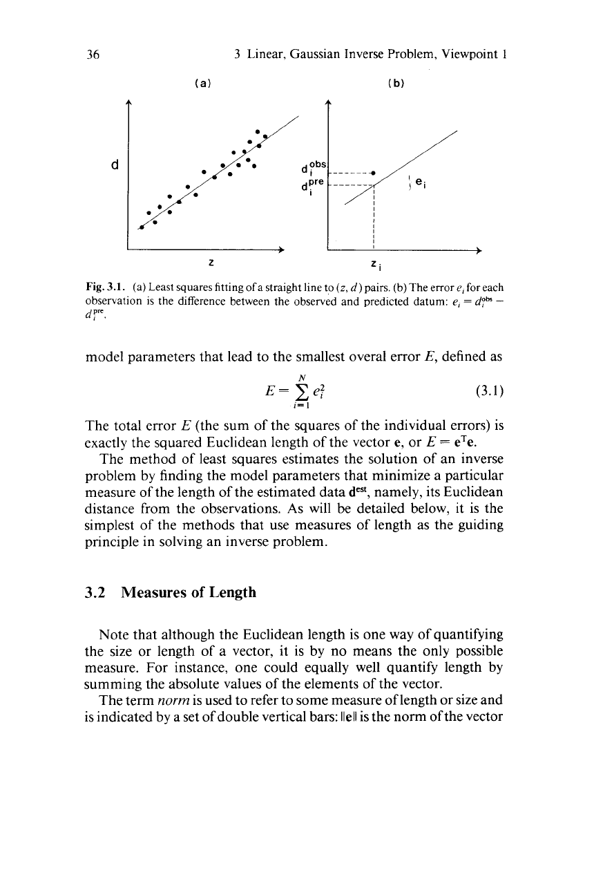
inverse problems, consider the simple problem of fitting a straight line
to data (Fig.
3.1).
This problem is often solved by the
so
called method
of least squares. In this method one tries to pick the model parameters
(intercept and slope)
so
that the predicted data are as close as possible
to the observed data. For each observation one defines a prediction
error, or misfit,
el
=
dpb”
-
dym.
The best fit-line is then the one with
35
36
3
Linear, Gaussian Inverse Problem,
Viewpoint
1
‘i
z
Fig.
3.1.
(a)
Least
squares fitting
ofa
straight line to
(z,
d)
pairs. (b) The error e, for each
observation
is
the difference between the observed and predicted datum: e,
=
dph
-
dy.
model parameters that lead to the smallest overal error
E,
defined as
N
E=
CeT
i-
I
The total error
E
(the sum of the squares of the individual errors) is
exactly the squared Euclidean length of the vector
e,
or
E
=
eTe.
The method of least squares estimates the solution of an inverse
problem by finding the model parameters that minimize a particular
measure of the length of the estimated data
dest,
namely, its Euclidean
distance from the observations.
As
will be detailed below, it
is
the
simplest of the methods that use measures of length as the guiding
principle in solving an inverse problem.
3.2
Measures
of
Length
Note that although the Euclidean length is one way of quantifying
the size or length of a vector, it is by no means the only possible
measure. For instance, one could equally well quantify length by
summing the absolute values of the elements of the vector.
The term
norm
is used to refer to some measure of length or size and
is indicated by a set of double vertical bars:
llell
is the norm of the vector
3.2
Measures
of
Length
37
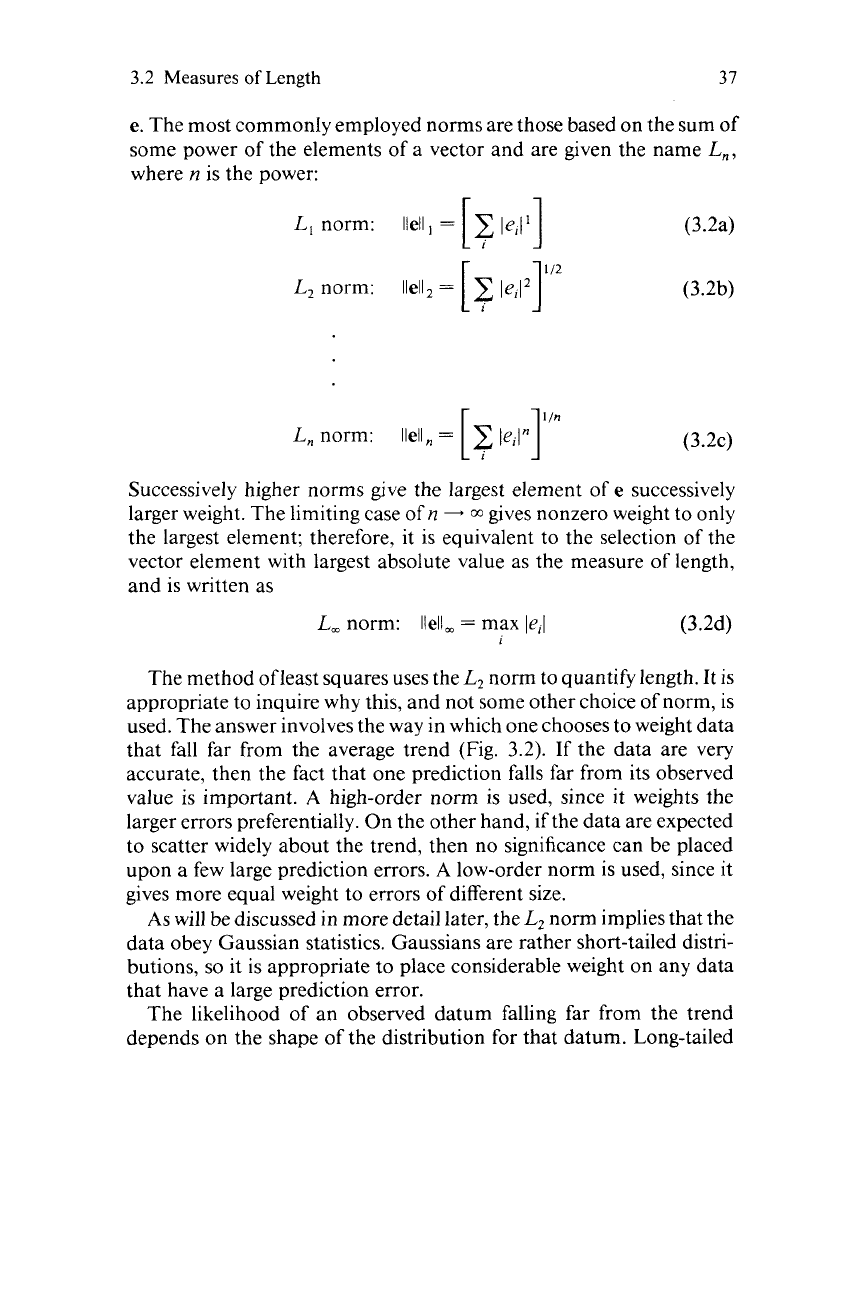
e.
The most commonly employed norms are those based on the sum of
some power of the elements of a vector and are given the name
L,,
where
n
is the power:
(3.2a)
(3.2~)
Successively higher norms give the largest element of
e
successively
larger weight. The limiting case of
n
-
~0
gives nonzero weight to only
the largest element; therefore, it is equivalent to the selection of the
vector element with largest absolute value as the measure of length,
and is written as
L,
norm:
llell,
=
max
le,l
(3.2d)
The method ofleast squares uses the
L,
norm to quantify length. It is
appropriate to inquire why this, and not some other choice of norm, is
used. The answer involves the way in which one chooses to weight data
that fall far from the average trend (Fig.
3.2).
If the data are very
accurate, then the fact that one prediction falls far from its observed
value
is
important.
A
high-order
norm
is used, since it weights the
larger errors preferentially. On the other hand, if the data are expected
to scatter widely about the trend, then no significance can be placed
upon a few large prediction errors.
A low-order norm is used, since it
gives more equal weight to errors of different size.
As
will be discussed in more detail later, the
L,
norm implies that the
data obey Gaussian statistics. Gaussians are rather short-tailed distri-
butions,
so it is appropriate to place considerable weight on any data
that have a large prediction error.
The likelihood of an observed datum falling far from the trend
depends on the shape of the distribution for that datum. Long-tailed
I