Menke W. Geophysical Data Analysis: Discrete Inverse Theory
Подождите немного. Документ загружается.

18
1
Describing Inverse Problems
1.4.1 ESTIMATES
OF
MODEL PARAMETERS
The simplist kind of solution to an inverse problem is an estimate
mest
of the model parameters. An estimate is simply a set of numerical
values for the model parameters,
mest
=
[1.4,
2.9,
. .
.
,
1.OIT
for example. Estimates are generally the most useful kind of solution
to an inverse problem. Nevertheless, in many situations they can be
very misleading. For instance, estimates in themselves gve no insight
into the quality of the solution. Depending on the structure of the
particular problem, measurement errors might be averaged out (in
which case the estimates might be meaningful) or amplified (in which
case the estimates might be nonsense). In other problems, many
solutions might exist. To single out arbitrarily only one of these
solutions and call it
mest
gives the false impression that a unique
solution has been obtained.
1.4.2 BOUNDING VALUES
One remedy to the problem of defining the quality
of
an estimate is
to state additionally some bounds that define its certainty. These
bounds can be either absolute or probabilistic. Absolute bounds imply
that the true value of the model parameter lies between two stated
values, for example,
1.3
5
m,
5
1.5.
Probabilistic bounds imply that
the estimate is likely to be between the bounds, with some given degree
of certainty. For instance,
myt
=
1.4
f
0.1
might mean that there is a
95%
probability that
my
lies between
1.3
and
1.5.
When they exist, bounding values can often provide the supplemen-
tary information needed to interpret properly the solution to an
inverse problem. There are, however, many instances in which
bounding values do not exist.
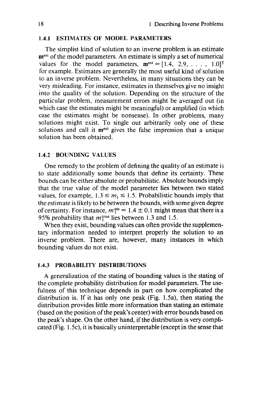
1.4.3 PROBABILITY DISTRIBUTIONS
A generalization
of
the stating of bounding values is the stating of
the complete probability distribution for model parameters. The use-
fulness of this technique depends in part
on
how complicated the
distribution is.
If
it has only one peak (Fig. 1.5a), then stating the
distribution provides little more information than stating an estimate
(based
on
the position of the peak’s center) with error bounds based
on
the peak’s shape. On the other hand,
if
the distribution is very compli-
cated (Fig.
1
Sc), it is basically uninterpretable (except in the sense that
1.4
Solutions to Inverse Problems
19
m1
m1 m1
Fig.
1.5.
Three probability distributions for a model parameter
M,
.
The first is
so
simple that its properties can be summarized by the central position and width
of
the
peak. The second implies that there are two probable ranges
for
the model parameter.
The third is
so
complicated that it provides
no
easily interpretable information about the
model parameter.
it implies that the model parameter cannot be well estimated). Only in
those exceptional instances in which the distribution has some inter-
mediate complexity (Fig. 1.5b) does it really provide information
toward the solution of an inverse problem. In practice, the most
interesting distributions are exceedingly difficult to compute,
so
this
technique is of rather limited usefulness.
1.4.4
WEIGHTED AVERAGES
OF
MODEL PARAMETERS
In many instances it is possible to identify combinations or averages
of the model parameters that are in some sense better determined than
the model parameters themselves. For instance, given
m
=
[m,
,
mJT
it may turn out that
(m)
=
0.24
+
0.8m,
is
better determined than
either
m,
or
m2.
Unfortunately, one might not have the slightest
interest in such an average, be it well determined or not, because it may
not have physical significance.
Averages
can
be of considerable interest when the model parameters
represent a discretized version
of
some continuous function.
If
the weights are
large only for a few physically adjacent parameters, then the average is said
to
be
localized. The meaning
of
the average in such a case is that, although
the data cannot resolve the model parameters at a particular point, they
can resolve the average
of
the model parameters
in
the neighborhood of
that point.

20
1
Describing Inverse Problems
In
the following chapters we shall derive methods for determining
each of these different kinds of solutions to inverse problems. We note
here, however, that there is a great deal
of
underlying similarity
between these types of “answers.” In fact, it will turn out that the same
numerical “answer” will be interpretable as any
of
several classes
of
solutions.
SOME COMMENTS
ON
PROBABILITY THEORY
2.1
Noise
and Random
Variables
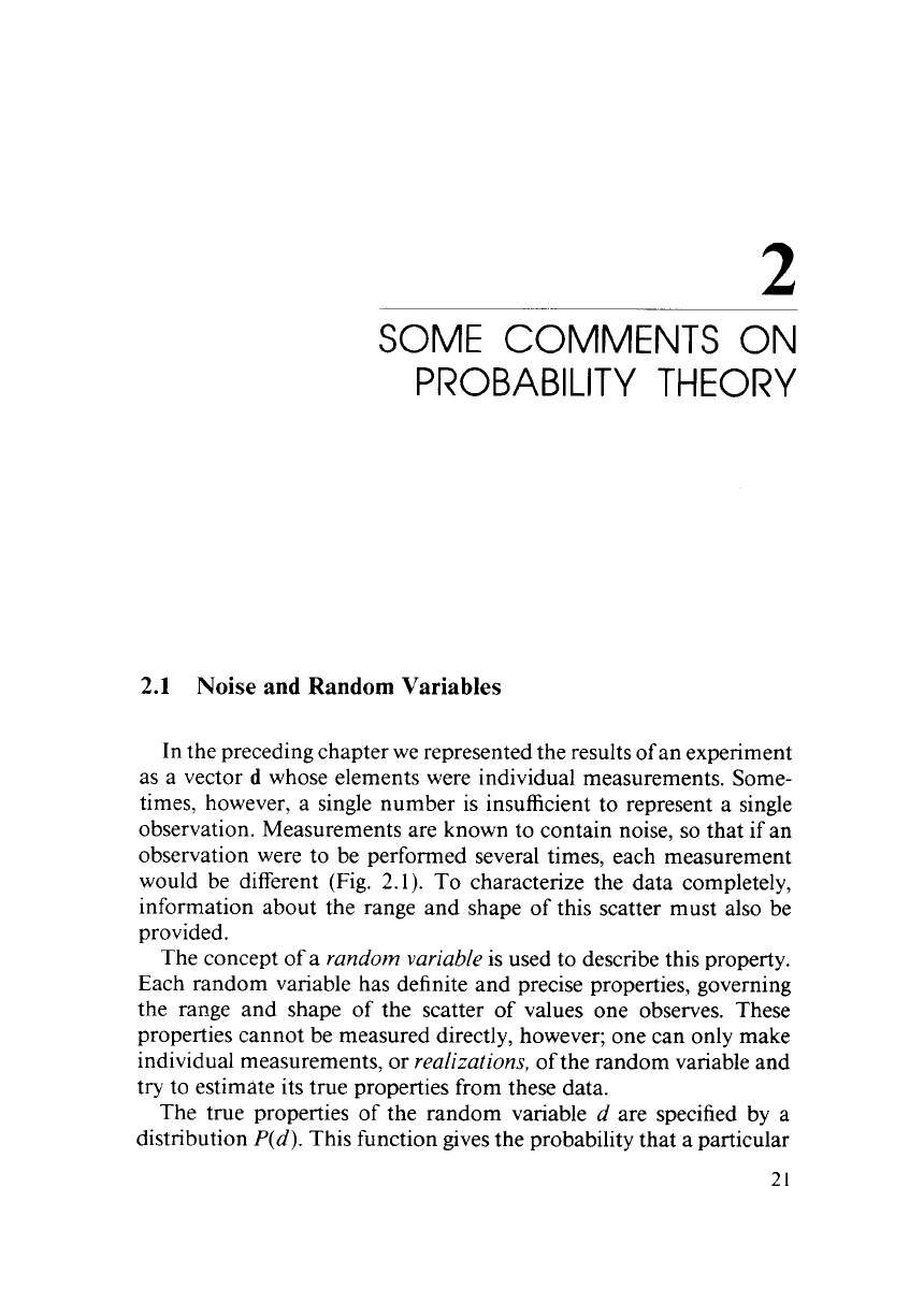
In the preceding chapter we represented the results of an experiment
as a vector
d
whose elements were individual measurements. Some-
times, however,
a
single number is insufficient to represent a single
observation. Measurements are known to contain noise,
so
that
if
an
observation were to be performed several times, each measurement
would be different (Fig.
2.1).
To characterize the data completely,
information about the range and shape of this scatter must also be
provided.
The concept
of
a
random variable
is used to describe this property.
Each random variable has definite and precise properties, governing
the range and shape of the scatter of values one observes. These
properties cannot be measured directly, however; one can only make
individual measurements, or
realizations,
of the random variable and
try to estimate its true properties from these data.
The true properties of the random variable
d
are specified by a
distribution
P(d).
This function gives the probability that a particular
21
22
2
Some
Comments
on
Probability
Theory
<d
>
datum d
Fig.
2.1.
Histogram showing data from
40
repetitions of an experiment. Noise causes
the data
to
scatter about their mean value
(d).
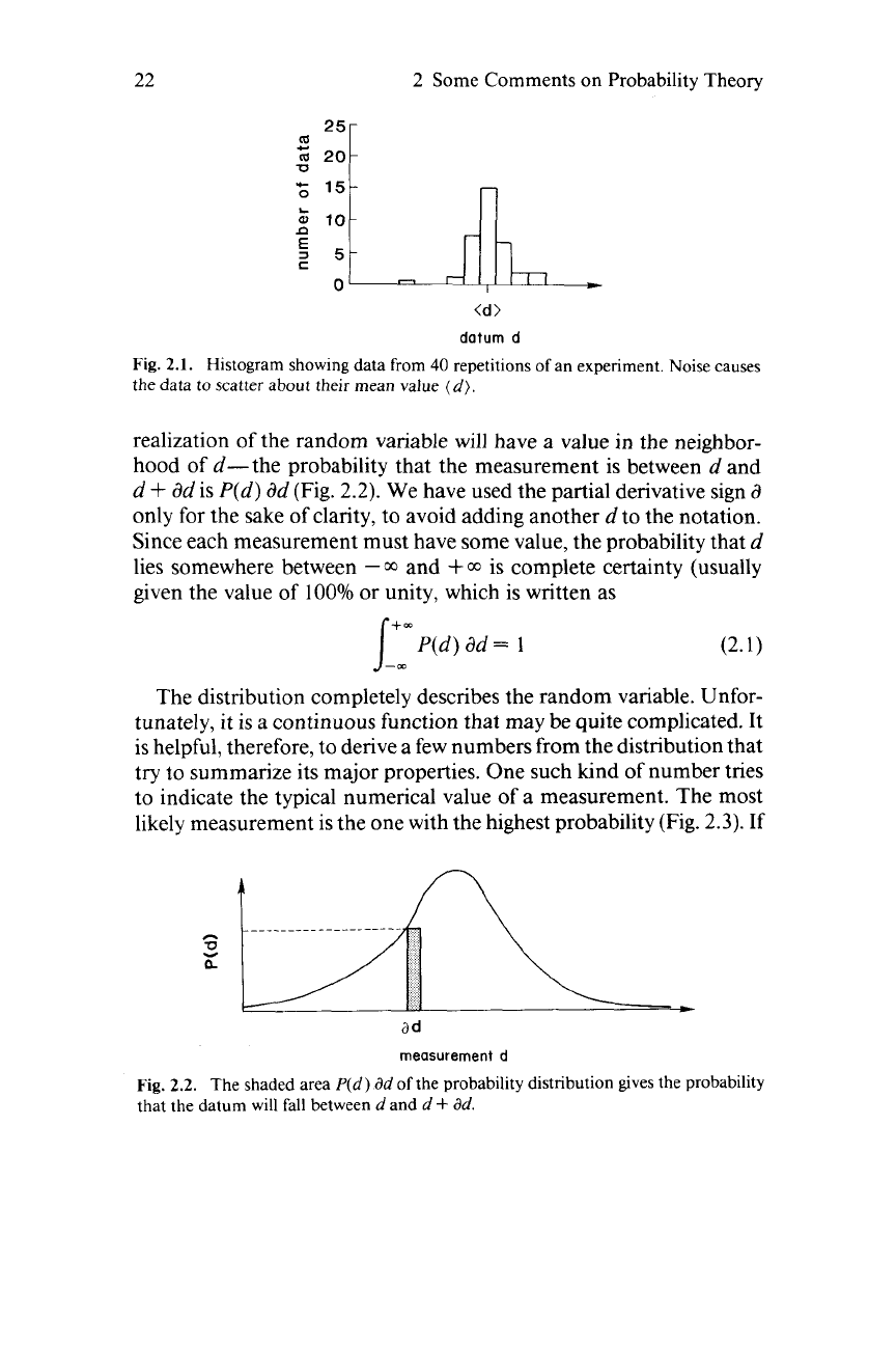
realization of the random variable will have a value
in
the neighbor-
hood of
d-
the probability that the measurement is between
d
and
d
+
ad
is
P(d)
dd
(Fig.
2.2).
We have used the partial derivative sign
d
only for the sake of clarity, to avoid adding another
d
to the notation.
Since each measurement must have some value, the probability that
d
lies somewhere between
-to
and
+
00
is complete certainty (usually
given the value of
100%
or
unity, which is written as
The distribution completely describes the random variable. Unfor-
tunately,
it
is a continuous function that may be quite complicated. It
is helpful, therefore, to derive a few numbers from the distribution that
try
to summarize its major properties. One such kind of number tries
to indicate the typical numerical value of a measurement. The most
likely measurement is the one with the highest probability (Fig.
2.3).
If
ad
measurement
d
Fig.
2.2.
The shaded area
P(d)
ad
of the probability distribution gives the probability
that the datum will fall between
d
and
d
+
ad.
2.1
Noise and Random Variables
23
measurement
d
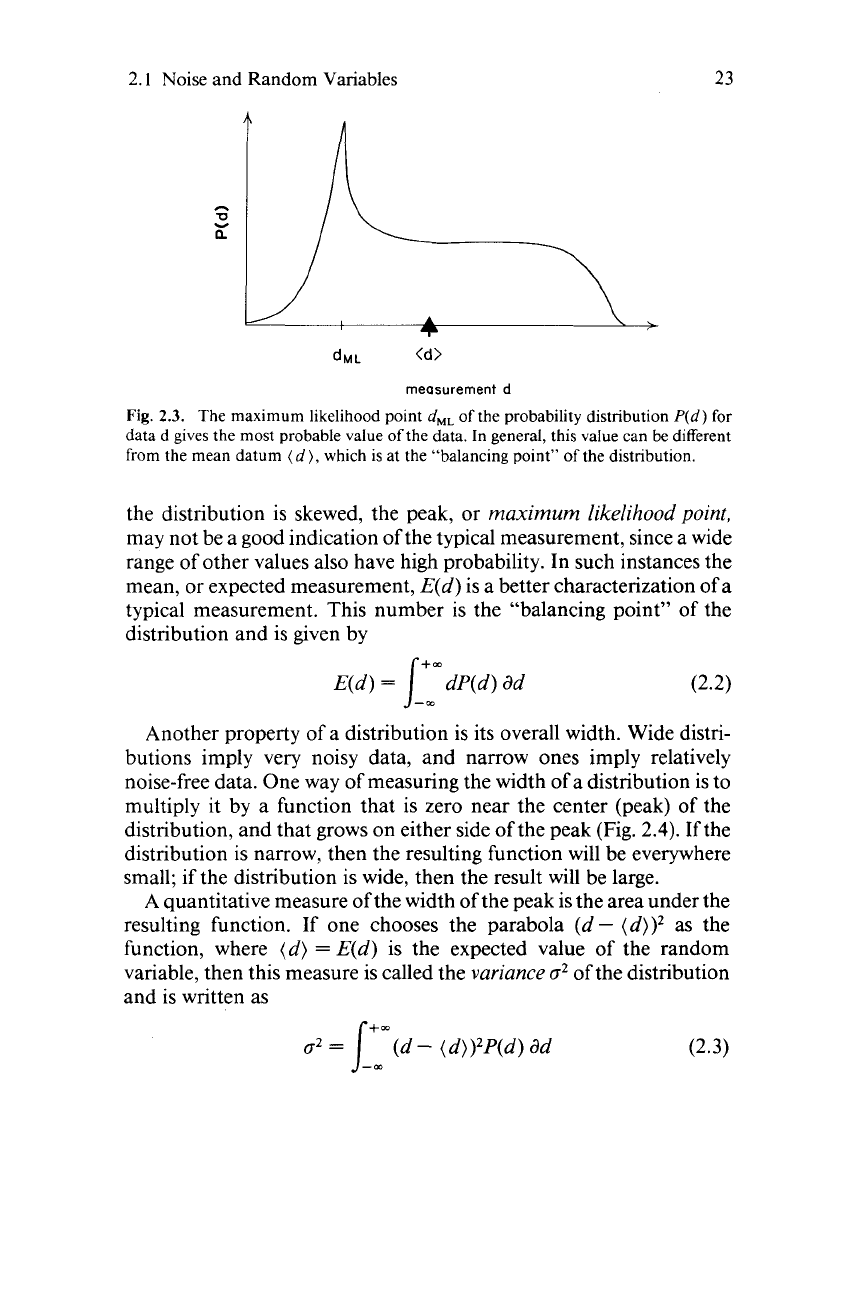
Fig.
2.3.
The maximum likelihood point
dML
of
the probability distribution
P(d)
for
data d gives the most probable value of the data. In general, this value can be different
from the mean datum (d), which
is
at the “balancing point”
of
the distribution.
the distribution is skewed, the peak, or
maximum likelihood point,
may not be a good indication of the typical measurement, since a wide
range of other values also have high probability. In such instances the
mean, or expected measurement,
E(d)
is a better characterization of a
typical measurement. This number is the “balancing point” of the
distribution and is given by
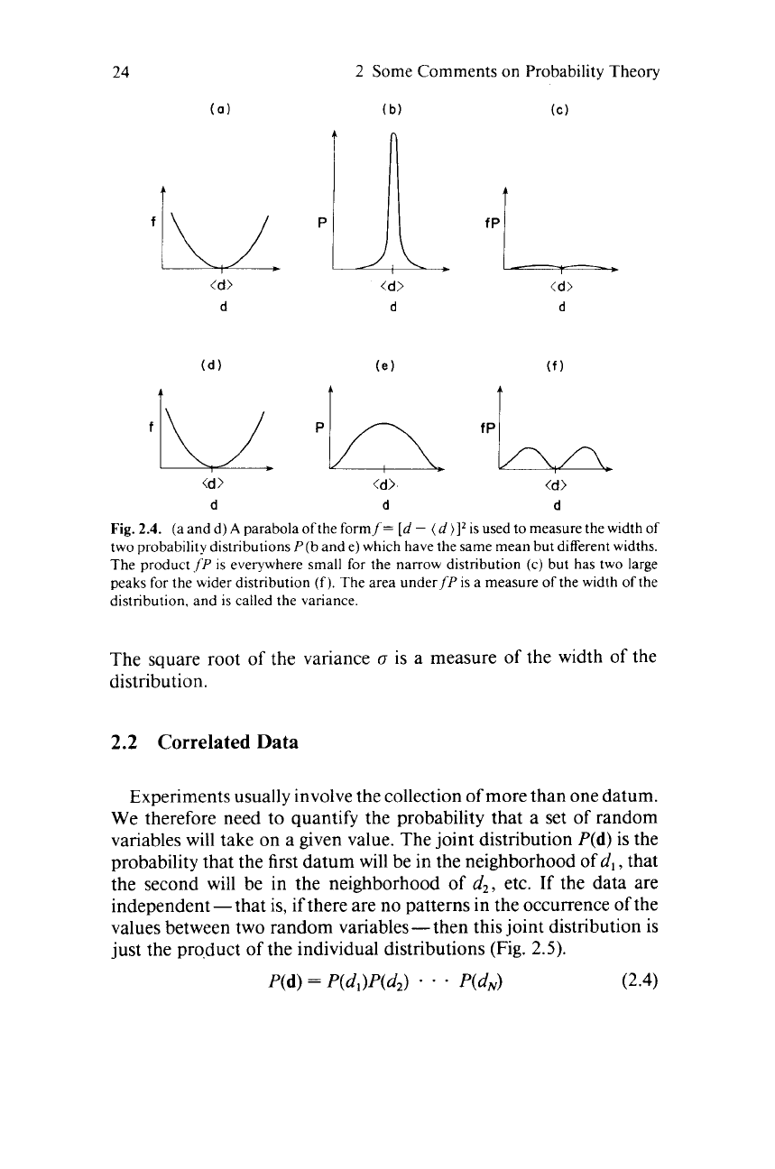
Another property of a distribution is its overall width. Wide distri-
butions imply very noisy data, and narrow ones imply relatively
noise-free data. One way of measuring the width
of
a distribution is to
multiply it by a function that is zero near the center (peak) of the
distribution, and that grows on either side of the peak (Fig.
2.4).
If the
distribution is narrow, then the resulting function will be everywhere
small; if the distribution is wide, then the result will be large.
A quantitative measure of the width of the peak is the area under the
resulting function. If one chooses the parabola
(d-
(d))2
as the
function, where
(d)
=
E(d)
is the expected value of the random
variable, then this measure is called the
variance
c2
of the distribution
and is written as
+-
a2
=
1-
(d
-
(d))2P(d)
ad
(2.3)
24
2
Some Comments
on
Probability
Theory
(a)
(b)
(C)
fL
<d>
d
pII
<d>
d
fpL
<d>
d
<d
>
<d>
<d
>
d d d
Fig. 2.4.
(a
and d)
A
parabola ofthe formf=
[d
-
(d)]*
is used to measure the width of
two probability distributions
P(b
and e) which have the same mean but different widths.
The product
.fP
is
everywhere small
for
the narrow distribution (c) but has two large
peaks
for the wider distribution
(f).
The area underfP
is
a
measure
of
the width
of
the
distribution. and
is
called the variance.
The square root
of
the variance
o
is a measure of the width
of
the
distribution.
2.2
Correlated Data
Experiments usually involve the collection
of
more than one datum.
We therefore need to quantify the probability that a set of random
variables will take on a given value. The joint distribution
P(d)
is the
probability that the first datum will be in the neighborhood of
d,
,
that
the second will be in the neighborhood
of
d,,
etc.
If
the data are
independent
-
that is, if there are no patterns in the occurrence
of
the
values between two random variables- then this joint distribution
is
just the prqduct of the individual distributions (Fig.
2.5).
P(
d)
=
P( d, )P(
d,)
-
*
-
P(
dN)
(2.4)
2.2
Correlated Data
d2
25
dl
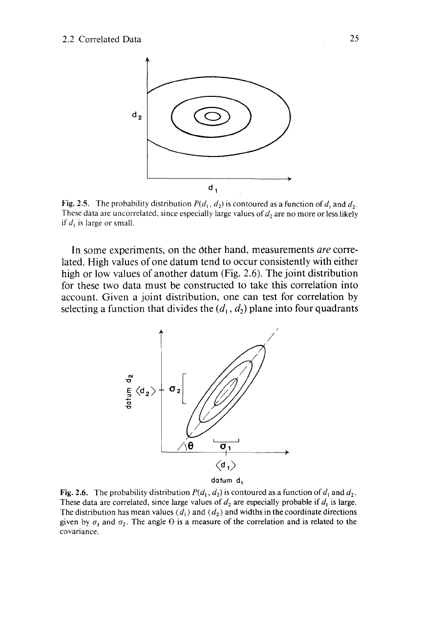
Fig.
2.5. The probability distribution
P(d,,
d,) is contoured as a function
of
d, and d,
These data are uncorrelated, since especially large values
of
d, are
no
more
or
less likely
if
d,
is
large
or
small.
In some experiments, on the &her hand, measurements
are
corre-
lated. High values of one datum tend to occur consistently with either
high or low values of another datum (Fig.
2.6).
The joint distribution
for these two data must be constructed to take this correlation into
account. Given a joint distribution, one can test for correlation by
selecting a function that divides the
(d,
,
d2)
plane into four quadrants
/'
datum
d,
Fig.
2.6.
The probability distribution
P(d,
,
d,)
is contoured as a function of
d,
and d,.
These data are correlated, since large values
of
d,
are especially probable if d, is large.
The distribution has mean values (d,
)
and (d,) and widths in the coordinate directions
given by
0,
and
a,.
The angle
0
is a measure
of
the correlation and is related to the
covariance.
26
I
I
I+
2
Some
Comments on
Probability
Theory
N
I
I
I
I+
-
d2
---~
@-
I
<dl>
dotum
d,
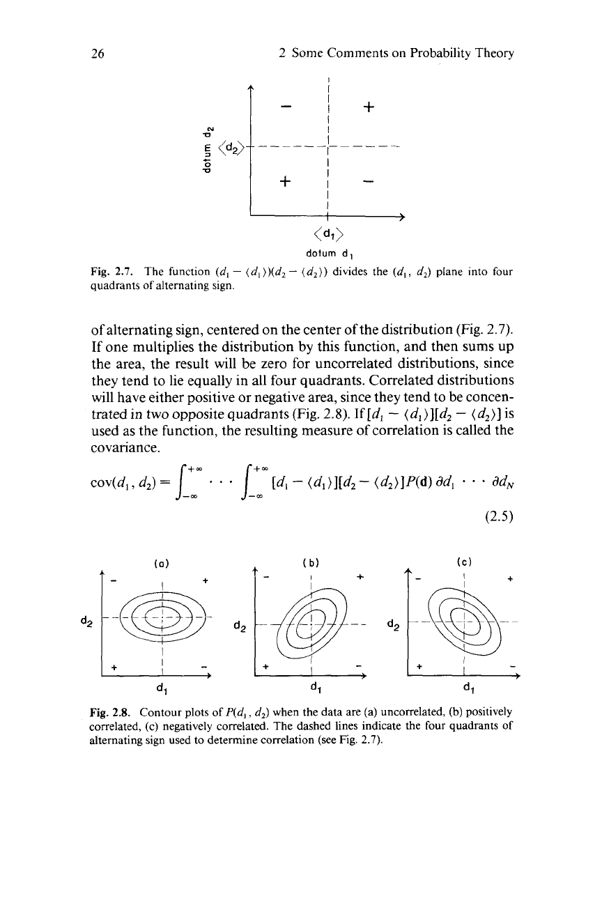
The function (d,
-
(d,))(d2
-
(d,))
divides the
(d,, d,)
plane into
four
Fig.
2.7.
quadrants
of
alternating sign.
of alternating sign, centered
on
the center
of
the distribution (Fig.
2.7).
If one multiplies the distribution by this function, and then sums up
the area, the result will be zero for uncorrelated distributions, since
they tend to lie equally in all four quadrants. Correlated distributions
will have either positive or negative area, since they tend to be concen-
trated in two opposite quadrants (Fig.
2.8).
If
[dl
-
(d,)
J[dz
-
(d,)]
is
used as the function, the resulting measure of correlation is called the
covariance.
cov(d,
,
dJ
=
[+-
.
[+-
[d,
-
(dl)j[d2
-
(d,)lP(d)
ad,
-
.
.
ad,
J--m
(0)
t-
I
+
+
I
I
-
b
J--m
d2
I
+
-
(C)
-
+
Fig.
2.8.
Contour plots
of
P(d,
,
d2)
when the data are (a) uncorrelated,
(b)
positively
correlated, (c) negatively correlated. The dashed lines indicate the
four
quadrants of
alternating sign used to determine correlation (see Fig.
2.7).
2.3
Functions
of
Random
Variables
27
Note that the covariance of a datum with itself is just the variance. The
covariance, therefore, characterizes the basic shape of joint distribu-
tion.
When there are many data given by the vector d, it is convenient
to
define a vector of expected values and a matrix of covariances as
(d)j
=
/+-mdd,
--m
/'mddz
-m
*
-
/-yddN
diP(d)
(2.6)
[cov
dIjj
=
-
*
-
rddN
[di
-
(d)J[d,
-
(d),]P(d)
The diagonal elements of the covariance matrix are a measure of the
width of the distribution of the data, and the off-diagonal elements
indicate the degree to which pairs of data are correlated.
--m
-m
2.3
Functions
of
Random Variables
The basic premise of inverse theory is that the data and model
parameters are related. Any method that solves the inverse problem
-that estimates a model parameter on the basis of data-will, there-
fore, tend to map errors from the data to the estimated model parame-
ters. Thus the
estimates
of the model parameters are themselves
random variables, which are described by a distribution
P(m").
Whether or not the
true
model parameters are random variables
depends on the problem. It is appropriate to consider them determi-
nistic quantities in some problems, and random variables in others.
Estimates of the parameters, however, are always random variables.
If
the distribution of the data is known, then the distribution for any
function of the data, including estimated model parameters, can be
found. Consider two uncorrelated data that are known to have white
distributions on the interval
[0,
I],
that is, they can take on any value
between
0
and
1
with equal probability (Fig. 2.9a). Suppose that some
model parameter is estimated to be the sum of these two data,
rn,
=
d,
+
dz.
The probability of this sum taking any particular value is
determined by identifying curves of equal
m,
in the
(d,,
dz)
plane and
integrating the distribution along these curves (Fig. 2.9b). Since in this
case
P(d)
is constant and the curves are straight lines,
P(rn,)
is just
a
triangular distribution on the interval
[0,
21 (Fig. 2.9~).