McConnell С., Campbell R. Macroeconomics: principles, problems, and policies, 17th ed

Подождите немного. Документ загружается.

CHAPTER 11

Fiscal Policy, Deficits, and Debt

213

proportional tax system , the average tax rate remains

constant as GDP rises. In a regressive tax system , the

average tax rate falls as GDP rises. The progressive tax

system has the steepest tax line T of the three. However,

tax revenues will rise with GDP under both the progres-

sive and the proportional tax systems, and they may rise,

fall, or stay the same under a regressive tax system. The

main point is this: The more progressive the tax system,

the greater the economy’s built-in stability.

The built-in stability provided by the U.S. tax system

has reduced the severity of business fluctuations, perhaps

by as much as 8 to 10 percent of the change in GDP that

otherwise would have occurred.

But built-in stabilizers

can only diminish, not eliminate, swings in real GDP. Dis-

cretionary fiscal policy (changes in tax rates and expendi-

tures) or monetary policy (central bank–caused changes in

interest rates) may be needed to correct recession or infla-

tion of any appreciable magnitude.

Evaluating Fiscal Policy

How can we determine whether discretionary fiscal policy

is expansionary, neutral, or contractionary in a particular

period? We cannot simply examine changes in the actual

budget deficits or surpluses, because those changes may

reflect automatic changes in tax revenues that accompany

changes in GDP, not changes in discretionary fiscal policy.

Moreover, the strength of any deliberate change in gov-

ernment spending or taxes depends on how large it is

relative to the size of the economy. So, in evaluating the

status of fiscal policy, we must adjust deficits and surpluses

to eliminate automatic changes in tax revenues and com-

pare the sizes of the adjusted budget deficits (or surpluses)

to the levels of potential GDP.

Standardized Budget

Economists use the standardized budget (also called the

full-employment budget ) to adjust the actual Federal budget

deficits and surpluses to eliminate the automatic changes

in tax revenues. The standardized budget measures what

the Federal budget deficit or surplus would be with exist-

ing tax rates and government spending levels if the econ-

omy had achieved its full-employment level of GDP (its

potential output) in each year. The idea essentially is to

compare actual government expenditures for each year

with the tax revenues that would have occurred in that year if

the economy had achieved full-employment GDP. That

procedure removes budget deficits or surpluses that arise

simply because of changes in GDP and thus tell us noth-

ing about changes in discretionary fiscal policy.

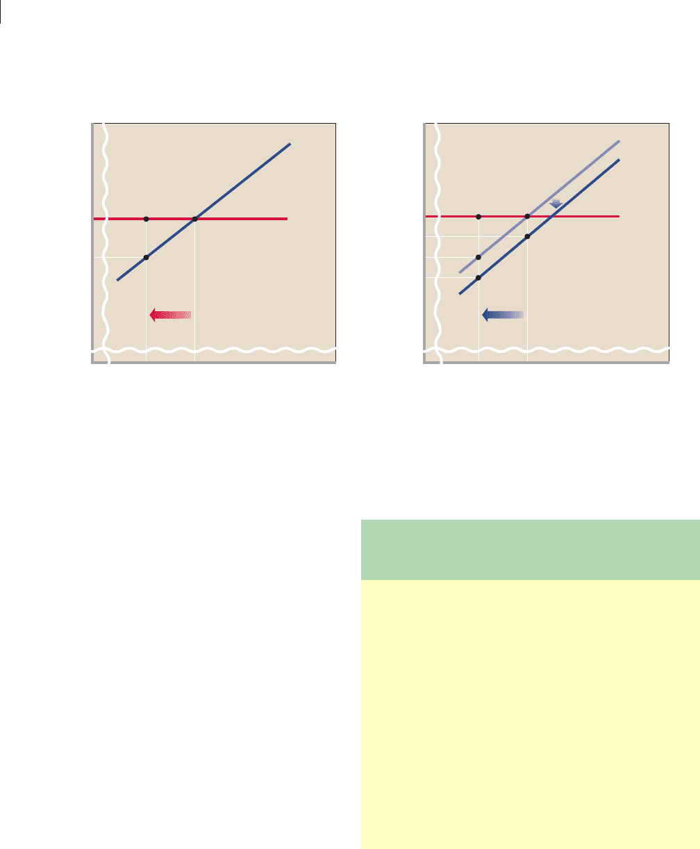
Consider Figure 11.4 a, where line G represents

government expenditures and line T represents tax reve-

nues. In full-employment year 1, government expenditures

of $500 billion equal tax revenues of $500 billion, as indi-

cated by the intersection of lines G and T at point a . The

standardized budget deficit in year 1 is zero—government

expenditures equal the tax revenues forthcoming at the

full-employment output GDP

. Obviously, the

full-employment deficit as a percentage of potential GDP is

also zero.

Now suppose that a recession occurs and GDP falls

from GDP

to GDP

, as shown in Figure 11.4 a. Let’s also

assume that the government takes no discretionary ac-

tion, so lines G and T remain as shown in the figure. Tax

revenues automatically fall to $450 billion (point c ) at

GDP

, while government spending remains unaltered at

$500 billion (point b) . A $50 billion budget deficit (repre-

sented by distance bc ) arises. But this cyclical deficit is

simply a by-product of the economy’s slide into recession,

not the result of discretionary fiscal actions by the gov-

ernment. We would be wrong to conclude from this defi-

cit that the government is engaging in an expansionary

fiscal policy.

That fact is highlighted when we consider the stan-

dardized budget deficit for year 2 in Figure 11.4 a. The

$500 billion of government expenditures in year 2 is shown

by b on line G . And, as shown by a on line T, $500 billion

of tax revenues would have occurred if the economy had

achieved its full-employment GDP. Because both b and a

represent $500 billion, the standardized budget deficit in

year 2 is zero, as is this deficit as a percentage of potential

GDP. Since the standardized deficits are zero in both

years, we know that government did not change its discre-

tionary fiscal policy, even though a recession occurred and

an actual deficit of $50 billion resulted.

Next, consider Figure 11.4 b. Suppose that real output

declined from full-employment GDP

to GDP

. But also

suppose that the Federal government responded to the re-

cession by reducing tax rates in year 4, as represented by

the downward shift of the tax line from T

to T

. What has

happened to the size of the standardized deficit? Govern-

ment expenditures in year 4 are $500 billion, as shown by

e . We compare that amount with the $475 billion of tax

revenues that would occur if the economy achieved its

full-employment GDP. That is, we compare position e on

line G with position h on line T

. The $25 billion of tax

revenues by which e exceeds h is the standardized budget

deficit for year 4. As a percentage of potential GDP, the

Alan J. Auerbach and Daniel Feenberg, “The Significance of Federal

Taxes as Automatic Stabilizers,” Journal of Economic Perspectives , Summer

2000, p. 54.

mcc26632_ch11_208-226.indd 213mcc26632_ch11_208-226.indd 213 8/21/06 4:35:12 PM8/21/06 4:35:12 PM

CONFIRMING PAGES

PART THREE

Macroeconomic Models and Fiscal Policy

214

standardized budget deficit has increased from zero in

year 3 (before the tax-rate cut) to some positive percent

[⫽ ( $25 billion 兾GDP

) ⫻ 100] in year 4. This increase in

the relative size of the full-employment deficit between

the two years reveals that fiscal policy is expansionary .

In contrast, if we observed a standardized deficit (as a

percentage of potential GDP) of zero in one year, followed

by a standardized budget surplus in the next, we could

conclude that fiscal policy is contractionary. Because the

standardized budget adjusts for automatic changes in tax

revenues, the increase in the standardized budget surplus

reveals that government either decreased its spending ( G )

or increased tax rates such that tax revenues ( T ) increased.

These changes in G and T are precisely the discretionary

actions that we have identified as elements of a contraction-

ary fiscal policy.

Recent U.S. Fiscal Policy

Table 11.1 lists the actual Federal budget deficits and

surpluses (column 2) and the standardized deficits and sur-

pluses (column 3), as percentages of actual and potential

GDP, respectively, for recent years. Observe that the stan-

dardized deficits are generally smaller than the actual

deficits. This is because the actual deficits include cyclical

$500

450

Government expenditures, G, and

tax revenues, T (billions)

Real domestic output, GDP

(a)

Zero standardized deficits,

years 1 and 2

GDP

(year 2)

GDP

(year 1)

$500

450

425

475

Government expenditures, G, and

tax revenues, T (billions)

Real domestic output, GDP

(b)

Zero standardized deficit, year 3;

$25 billion full-employment deficit, year 4

GDP

(year 4)

GDP

(year 3)

FIGURE 11.4 Standardized deficits. (a) In the left-hand graph the standardized deficit is zero at the full-employment output GDP

. But it is also

zero at the recessionary output GDP

, because the $500 billion of government expenditures at GDP

equals the $500 billion of tax revenues that would be

forthcoming at the full-employment GDP

. There has been no change in fiscal policy. (b) In the right-hand graph, discretionary fiscal policy, as reflected in the

downward shift of the tax line from T

to T

, has increased the standardized budget deficit from zero in year 3 to $25 billion in year 4. This is found by comparing

the $500 billion of government spending in year 4 with the $475 billion of taxes that would accrue at the full-employment GDP

. Such a rise in the standardized deficit

(as a percentage of potential GDP) identifies an expansionary fiscal policy.

TABLE 11.1 Federal Deficits (ⴚ) and Surpluses (ⴙ) as

Percentages of GDP, 1990–2005

*As a percentage of potential GDP.

Source: Congressional Budget Office, www.cbo.gov .

(2) (3)

Actual Standardized

(1) Deficit ⴚ or Deficit ⴚ or

Year Surplus ⴙ Surplus ⴙ *

1990 ⫺3.9% ⫺2.2%

1991 ⫺4.4 ⫺2.5

1992 ⫺4.5 ⫺2.9

1993 ⫺3.8 ⫺2.9

1994 ⫺2.9 ⫺2.1

1995 ⫺2.2 ⫺2.0

1996 ⫺1.4 ⫺1.2

1997 ⫺0.3 ⫺1.0

1998 ⫹0.8 ⫺0.4

1999 ⫹1.4 ⫹0.1

2000 ⫹2.5 ⫹1.1

2001 ⫹1.3 ⫹1.1

2002 ⫺1.5 ⫺1.1

2003 ⫺3.4 ⫺2.7

2004 ⫺3.5 ⫺2.4

2005 ⫺2.6 ⫺1.8

mcc26632_ch11_208-226.indd 214mcc26632_ch11_208-226.indd 214 8/21/06 4:35:12 PM8/21/06 4:35:12 PM

CONFIRMING PAGES

CHAPTER 11

Fiscal Policy, Deficits, and Debt

215

deficits, whereas the standardized deficits do not. The lat-

ter deficits provide the information needed to assess dis-

cretionary fiscal policy.

Column 3 shows that fiscal policy was expansionary in

the early 1990s. Consider 1992, for example. From the ta-

ble we see that the actual budget deficit was 4.5 percent of

GDP and the standardized budget deficit was 2.9 percent

of potential GDP. The economy was recovering from the

1990–1991 recession, so tax revenues were relatively low.

But even if the economy were at full employment in 1992,

with the greater tax revenues that would imply, the Federal

budget would have been in deficit by 2.9 percent. And that

percentage was greater than the deficits in the prior 2

years. So the standardized budget deficit in 1992 clearly

reflected expansionary fiscal policy.

But the large standardized budget deficits were pro-

jected to continue even when the economy fully recovered

from the 1990–1991 recession. The concern was that the

large actual and standardized deficits would cause high in-

terest rates, low levels of investment, and slow economic

growth. In 1993 the Clinton administration and Congress

increased personal income and corporate income tax rates

to prevent these potential outcomes. Observe from col-

umn 3 of Table 11.1 that the standardized budget deficits

shrunk each year and eventually gave way to surpluses in

1999, 2000, and 2001.

On the basis of projections that actual budget sur-

pluses would accumulate to as much as $5 trillion between

2000 and 2010, the Bush administration and Congress

passed a major tax reduction package in 2001. The tax cuts

went into effect over a number of years. For example, the

cuts reduced tax liabilities by an estimated $44 billion in

2001 and $52 billion in 2002. In terms of fiscal policy, the

timing was good since the economy entered a recession in

March 2001 and absorbed a second economic blow from

the terrorist attacks on September 11, 2001. The govern-

ment greatly increased its spending on war abroad and

homeland security. Also, in March 2002 Congress passed a

“recession-relief” bill that extended unemployment com-

pensation benefits and offered business tax relief. That

legislation was specifically designed to inject $51 billion

into the economy in 2002 and another $71 billion over the

following 2 years.

As seen in Table 11.1 , the standardized budget moved

from a surplus of 1.1 percent of potential GDP in 2000 to a

deficit of 1.1 percent in 2002. Clearly, fiscal policy had turned

expansionary. Nevertheless, the economy remained very

sluggish in 2003. In June of that year, Congress again cut

taxes, this time by an enormous $350 billion over several

years. Specifically, the tax legislation accelerated the reduc-

tion of marginal tax rates already scheduled for future years

and slashed tax rates on income from dividends and capital

gains. It also increased tax breaks for families and small busi-

nesses. This tax package increased the standardized budget

deficit as a percentage of potential GDP to –2.7 percent in

2003. The purpose of this expansionary fiscal policy was to

prevent another recession, reduce unemployment, and

increase economic growth. (Key Question 6)

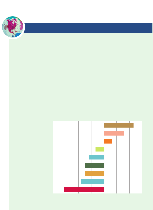
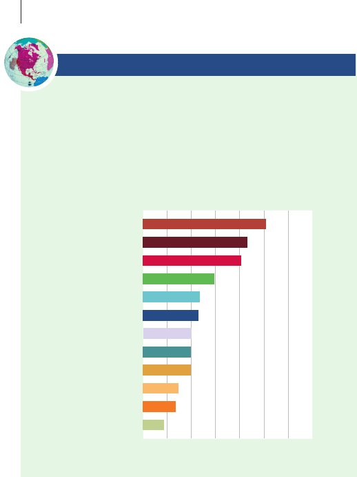
Global Perspective 11.1 shows the extent of the stan-

dardized deficits or surpluses of a number of countries in a

recent year.

Budget Deficits and Projections

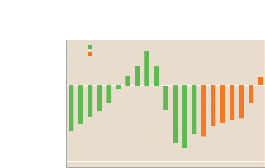
Figure 11.5 shows the absolute magnitudes of recent U.S.

budget surpluses and deficits. It also shows the projected

future deficits or surpluses as published by the Congres-

sional Budget Office (CBO). The United States has been

experiencing large budget deficits that are expected to

continue for several years. But projected deficits and sur-

pluses are subject to swift change, as government alters its

fiscal policy and the GDP growth accelerates or slows. So

we suggest that you update this figure by going to the

GLOBAL PERSPECTIVE 11.1

Standardized Budget Deficits or Surpluses as a

Percentage of Potential GDP, Selected Nations

In 2005 some nations had standardized budget surpluses, while

others had standardized budget deficits. These surpluses and

deficits varied as a percentage of each nation’s potential GDP.

Generally, the surpluses represented contractionary fiscal pol-

icy and the deficits expansionary fiscal policy.

Source: Organization for Economic Cooperation and Development,

www.oecd.org .

Standardized Budget Surplus

or Deficit as a Percentage of

Potential GDP, 2005

Deficits Surpluses

⫺4⫺6⫺8 ⫺20 4 62

New Zealand

Denmark

Canada

Ireland

France

Norway

United Kingdom

United States

Japan

mcc26632_ch11_208-226.indd 215mcc26632_ch11_208-226.indd 215 8/21/06 4:35:13 PM8/21/06 4:35:13 PM

CONFIRMING PAGES

PART THREE

Macroeconomic Models and Fiscal Policy

216

Congressional Budget Office Web site, www.cbo.gov ,

and selecting Current Budget Projections and then CBO’s

Baseline Budget Projections. The relevant numbers are in

the row Surplus (⫹) or Deficit (⫺).

Social Security Considerations

The surpluses and deficits in Figure 11.5 include all tax

revenues, even those obligated for future Social Security

payments. Recall from the Last Word in Chapter 4 that

Social Security is basically a “pay-as-you-go plan” in

which the mandated benefits paid out each year are fi-

nanced by the payroll tax revenues received each year. But

current tax rates now bring in more revenue than current

payouts, in partial preparation for the opposite circum-

stance when the baby boomers retire in the next one or

two decades. The Federal government saves the excess

revenues by purchasing U.S. securities and holding them

in the Social Security trust fund.

Some economists argue that these present Social Se-

curity surpluses ($175 billion in 2005) should be subtracted

from Federal government revenue when calculating pres-

ent Federal deficits. Because these surpluses represent fu-

ture government obligations on a dollar-for-dollar basis,

they should not be considered revenue offsets to current

government spending. Without the Social Security sur-

pluses, the total budget deficit in 2005 would be $523 bil-

lion rather than the $318 billion shown.

Problems, Criticisms, and

Complications

Economists recognize that governments may encounter a

number of significant problems in enacting and applying

fiscal policy.

Problems of Timing

Several problems of timing may arise in connection with

fiscal policy:

• Recognition lag The recognition lag is the time be-

tween the beginning of recession or inflation and the

certain awareness that it is actually happening. This

lag arises because of the difficulty in predicting the

future course of economic activity. Although fore-

casting tools such as the index of leading indicators

(see this chapter’s Last Word) provide clues to the

direction of the economy, the economy may be 4 or

6 months into a recession or inflation before that fact

appears in relevant statistics and is acknowledged.

Meanwhile, the economic downslide or the inflation

⫺200

⫺300

⫺400

⫺500

⫺100

100

200

1992 1994 1996 1998 2000 2002 2004 2006 2008 2010 2012

$300

Actual

Projected

(as of March 2006)

Budget deficit (ⴚ) or surplus, billions

Year

FIGURE 11.5 Federal budget deficits and surpluses, actual and projected, fiscal years 1992–

2012 (in billions of nominal dollars). The annual budget deficits of 1992 through 1997 gave way to budget surpluses

from 1998 through 2001. Deficits reappeared in 2002 and are projected to continue through 2011.

Source: Congressional Budget Office, www.cbo.gov .

mcc26632_ch11_208-226.indd 216mcc26632_ch11_208-226.indd 216 3/8/07 6:47:25 PM3/8/07 6:47:25 PM

CHAPTER 11

Fiscal Policy, Deficits, and Debt

217

Future Policy Reversals

Fiscal policy may fail to achieve its intended objectives if

households expect future reversals of policy. Consider a

tax cut, for example. If taxpayers believe the tax reduction

is temporary, they may save a large portion of their tax

saving, reasoning that rates will return to their previous

level in the future. At that time, they can draw on this ex-

tra saving to maintain their consumption. So a tax reduc-

tion thought to be temporary may not increase present

consumption spending and aggregate demand by as much

as our simple model ( Figure 11.1 ) suggests.

The opposite may be true for a tax increase. If taxpay-

ers think it is temporary, they may reduce their saving to

pay the tax while maintaining their present consumption.

They may reason they can restore their saving when the

tax rate again falls. So the tax increase may not reduce cur-

rent consumption and aggregate demand by as much as

the policymakers desired.

To the extent that this so-called consumption smoothing

occurs over time, fiscal policy will lose some of its

strength. The lesson is that tax-rate changes that house-

holds view as permanent are more likely to alter consump-

tion and aggregate demand than tax changes they view as

temporary.

Offsetting State and Local

Finance

The fiscal policies of state and local governments are

frequently pro-cyclical, meaning that they worsen rather

than correct recession or inflation. Unlike the Federal

government, most state and local governments face

constitutional or other legal requirements to balance their

budgets. Like households and private businesses, state and

local governments increase their expenditures during

prosperity and cut them during recession. During the

Great Depression of the 1930s, most of the increase in

Federal spending was offset by decreases in state and local

spending. During and immediately following the recession

of 2001, many state and local governments had to increase

tax rates, impose new taxes, and reduce spending to offset

lower tax revenues resulting from the reduced personal

income and spending of their citizens.

Crowding-Out Effect

Another potential flaw of fiscal policy is the so-called

crowding-out effect : An expansionary fiscal policy (defi-

cit spending) may increase the interest rate and reduce pri-

vate spending, thereby weakening or canceling the stimulus

of the expansionary policy.

may become more serious than it would have if the

situation had been identified and acted on sooner.

• Administrative lag The wheels of democratic

government turn slowly. There will typically be a sig-

nificant lag between the time the need for fiscal ac-

tion is recognized and the time action is taken.

Following the terrorist attacks of September 11,

2001, the U.S. Congress was stalemated for 5 months

before passing a compromise economic stimulus law

in March 2002. (In contrast, the Federal Reserve be-

gan lowering interest rates the week after the attacks.)

• Operational lag A lag also occurs between the time

fiscal action is taken and the time that action affects

output, employment, or the price level. Although

changes in tax rates can be put into effect relatively

quickly, government spending on public works—new

dams, interstate highways, and so on—requires long

planning periods and even longer periods of con-

struction. Such spending is of questionable use in

offsetting short (for example, 6- to 12-month) peri-

ods of recession. Consequently, discretionary fiscal

policy has increasingly relied on tax changes rather

than on changes in spending as its main tool.

Political Considerations

Fiscal policy is conducted in a political arena. That reality not

only may slow the enactment of fiscal policy but also may

create the potential for political considerations swamping

economic considerations in its formulation. It is a human trait

to rationalize actions and policies that are in one’s self-interest.

Politicians are very human—they want to get reelected. A

strong economy at election time will certainly help them. So

they may favor large tax cuts under the guise of expansionary

fiscal policy even though that policy is economically

inappropriate. Similarly, they may rationalize increased

government spending on popular items such as farm subsidies,

health care, highways, education, and homeland security.

At the extreme, elected officials and political parties

might collectively “hijack” fiscal policy for political pur-

poses, cause inappropriate changes in aggregate demand,

and thereby cause (rather than avert) economic fluctua-

tions. They may stimulate the economy using expansion-

ary fiscal policy before elections and use contractionary

fiscal policy to dampen excessive aggregate demand after

the election. In short, elected officials may cause so-called

political business cycles . Such scenarios are difficult to

document and prove, but there is little doubt that political

considerations weigh heavily in the formulation of fiscal

policy. The question is how often, if ever, do those politi-

cal considerations run counter to “sound economics.”

mcc26632_ch11_208-226.indd 217mcc26632_ch11_208-226.indd 217 8/21/06 4:35:13 PM8/21/06 4:35:13 PM

CONFIRMING PAGES

PART THREE

Macroeconomic Models and Fiscal Policy

218

Suppose the economy is in recession

and government enacts a discretionary fis-

cal policy in the form of increased govern-

ment spending. Also suppose that the

monetary authorities hold the supply of

money constant. To finance its budget defi-

cit, the government borrows funds in the

money market. The resulting increase in

the demand for money raises the price paid for borrowing

money: the interest rate. Because investment spending

varies inversely with the interest rate, some investment will

be choked off or crowded out. (Some interest-sensitive

consumption spending such as purchases of automobiles

on credit may also be crowded out.)

Nearly all economists agree that a budget deficit is

inappropriate when the economy has achieved full

employment. Such a deficit will surely crowd out some

private investment. But economists disagree on whether

crowding out exists under all circumstances. Many believe

that little crowding out will occur when fiscal policy is

used to move the economy from recession. The added

amount of government financing resulting from typical

budget deficits is small compared to the total amount of

private and public financing occurring in the money

market. Therefore, interest rates are not likely to be

greatly affected. Moreover, both increased government

spending and increased consumption spending resulting

from tax cuts may improve the profit expectations of

businesses. The greater expected returns on private

investment may encourage more of it. Thus, private

investment need not fall, even though interest rates do

rise. (We will soon see that the financing of the entire

public debt, as opposed to the financing of new debt from

annual deficits, is more likely to raise interest rates.)

Current Thinking on Fiscal Policy

Where do these complications leave us as to the advisabil-

ity and effectiveness of discretionary fiscal policy? In view

of the complications and uncertain outcomes of fiscal pol-

icy, some economists argue that it is better not to engage

in it at all. Those holding that view point to the superior-

ity of monetary policy (changes in interest rates engi-

neered by the Federal Reserve) as a stabilizing device or

believe that most economic fluctuations tend to be mild

and self-correcting.

But most economists believe that fiscal policy remains

an important, useful policy lever in the government’s mac-

roeconomic toolkit. The current popular view is that fiscal

policy can help push the economy in a particular direction

but cannot fine-tune it to a precise macroeconomic outcome.

Mainstream economists generally agree that monetary

policy is the best month-to-month stabilization tool for the

U.S. economy. If monetary policy is doing its job, the gov-

ernment should maintain a relatively neutral fiscal policy,

with a standardized budget deficit or surplus of no more

than 2 percent of potential GDP. It should hold major dis-

cretionary fiscal policy in reserve to help counter situations

where recession threatens to be deep and long-lasting or

where inflation threatens to escalate rapidly despite the ef-

forts of the Federal Reserve to stabilize the economy.

Finally, economists agree that proposed fiscal policy

should be evaluated for its potential positive and negative

impacts on long-run productivity growth. The short-run

policy tools used for conducting active fiscal policy often

have long-run impacts. Countercyclical fiscal policy should

be shaped to strengthen, or at least not impede, the growth

of long-run aggregate supply (shown as a rightward shift of

the long-run aggregate supply curve in Figure 10.3). For

example, a tax cut might be structured to enhance work ef-

fort, strengthen investment, and encourage innovation. Al-

ternatively, an increase in government spending might

center on preplanned projects for public capital (highways,

mass transit, ports, airports), which are complementary to

private investment and thus support long-term economic

growth. (Key Question 8)

QUICK REVIEW 11.2

• Automatic changes in net taxes (taxes minus transfers) add a

degree of built-in stability to the economy.

• The standardized budget compares government spending to

the tax revenues that would accrue if there were full

employment; changes in standardized budget deficits or

surpluses (as percentages of potential GDP) reveal whether

fiscal policy is expansionary, neutral, or contractionary.

• Standardized budget deficits are distinct from cyclical

deficits, which simply reflect declines in tax revenues

resulting from reduced GDP.

• Time lags, political problems, expectations, and state and

local finances complicate fiscal policy.

• The crowding-out effect indicates that an expansionary fiscal

policy may increase the interest rate and reduce investment

spending.

O 11.2

Crowding out

The Public Debt

The national or public debt is essentially the total accu-

mulation of the deficits (minus the surpluses) the Federal

government has incurred through time. These deficits

have emerged mainly because of war financing, recessions,

and fiscal policy. Lack of political will by Congress has also

mcc26632_ch11_208-226.indd 218mcc26632_ch11_208-226.indd 218 8/21/06 4:35:13 PM8/21/06 4:35:13 PM

CONFIRMING PAGES

CHAPTER 11

Fiscal Policy, Deficits, and Debt

219

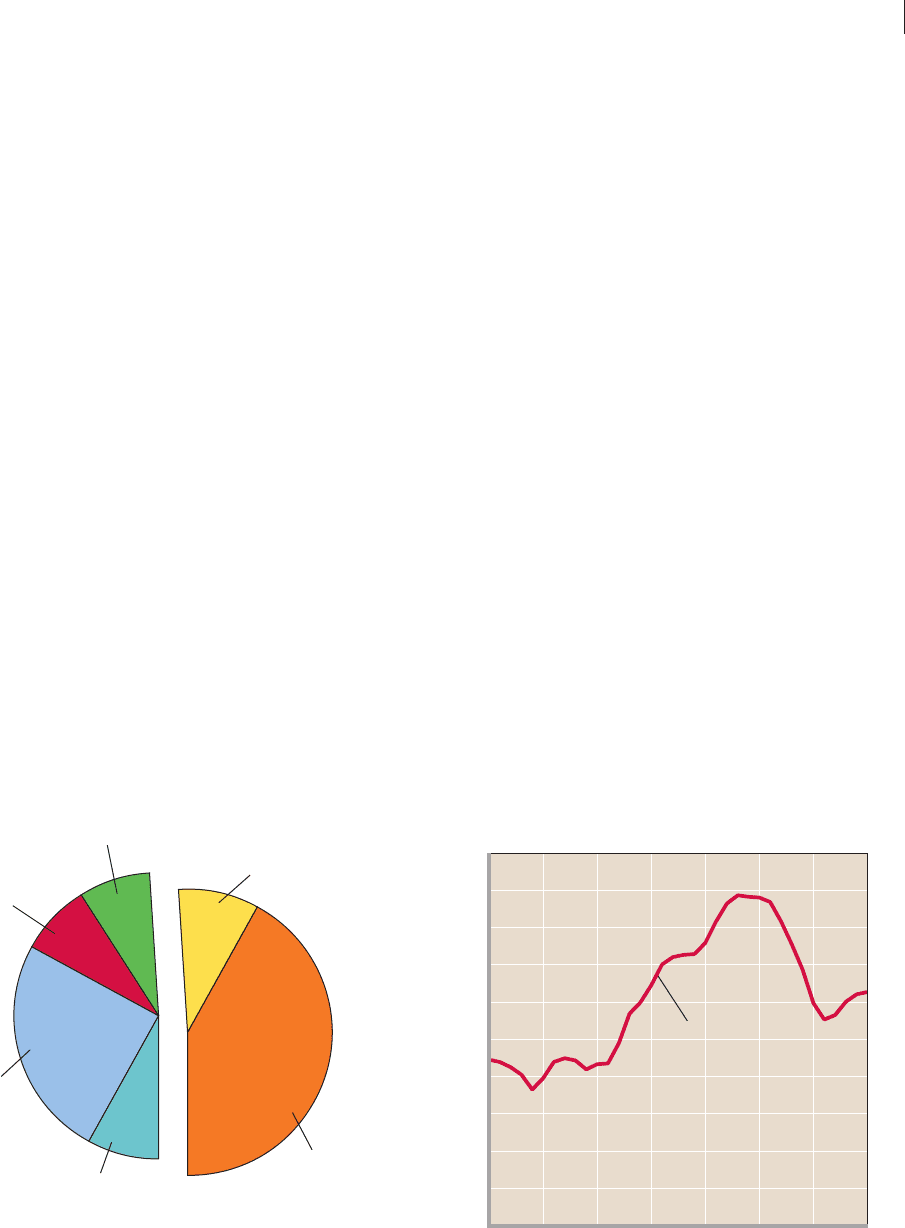
FIGURE 11.7 Federal debt held by the public as a

percentage of GDP, 1970–2005. As a percentage of GDP, the Federal

debt held by the public (held outside the Federal Reserve and Federal

government agencies) increased sharply over the 1980–1995 period and

declined significantly between 1995 and 2001. Since 2001, the percentage has

gone up again, but remains lower than it was in the 1990s.

Federal debt held

by the public as a

percentage of GDP

Percent of GDP

1970 1975 1980 1985 1990 1995 2000

2005

Year

contributed to the size of the debt. In 2005 the total public

debt was $7.96 trillion—$3.9 trillion held by the public and

$4.06 trillion held by Federal Agencies and the Federal Re-

serve. (You can find the size of the public debt, to the penny,

at the Web site of the Department of Treasury, Bureau

of the Public Debt, at www.publicdebt.treas.gov/opd/

opdpenny.htm .)

Ownership

The total public debt of nearly $8 trillion represents the

total amount of money owed by the Federal government

to the holders of U.S. securities : financial instruments

issued by the Federal government to borrow money to fi-

nance expenditures that exceed tax revenues. These U.S.

securities (loan instruments) are of four types: Treasury

bills (short-term securities), Treasury notes (medium-term

securities), Treasury bonds (long-term securities), and

U.S. saving bonds (long-term, nonmarketable bonds).

Figure 11.6 shows that the public held 49 percent of

the Federal debt in 2005 and that Federal government

agencies and the Federal Reserve (the U.S. central bank)

held the other 51 percent. In this case the “public” consists

of individuals here and abroad, state and local govern-

ments, and U.S. financial institutions. Foreigners held

about 25 percent of the total debt in 2005. So, most of the

debt is held internally, not externally. Americans owe

three-fourths of the debt to Americans.

Debt and GDP

A simple statement of the absolute size of the debt ignores

the fact that the wealth and productive ability of the U.S.

economy is also vast. A wealthy, highly productive nation

can incur and carry a large public debt more easily than a

poor nation can. A more meaningful measure of the public

debt relates it to an economy’s GDP. Figure 11.7 shows

the relative size of the Federal debt held by the public (as

opposed to the Federal Reserve and Federal agencies) over

time. This percentage—31.4 percent in 2005—has in-

creased since 2001, but remains well below the percent-

ages in the 1990s.

International Comparisons

As shown in Global Perspective 11.2, it is not uncommon

for countries to have public debts. The numbers shown

are government debts held by the public, as a percentage

of GDP.

FIGURE 11.6 Ownership of the total public debt, 2005.

The total public debt can be divided into the proportion held by the public

(49 percent) and the proportion held by Federal agencies and the Federal

Reserve System (51 percent). Of the total debt, 25 percent is foreign-

owned.

U.S.

individuals

Foreign

ownership

Other, including state

and local governments

Debt held outside the Federal

government and Federal

Reserve (49%)

Debt held by the Federal

government and Federal

Reserve (51%)

Total debt: $7.96 trillion

25%

42%

Federal

Reserve

U.S.

government

agencies

U.S. banks

and other

financial

institutions

Source: U.S. Treasury, www.fms.treas.gov/ bulletin.

mcc26632_ch11_208-226.indd 219mcc26632_ch11_208-226.indd 219 8/21/06 4:35:14 PM8/21/06 4:35:14 PM

CONFIRMING PAGES

PART THREE

Macroeconomic Models and Fiscal Policy

220

are false concerns. People were wondering the same things

50 years ago!

Bankruptcy

The large U.S. public debt does not threaten to bankrupt

the Federal government, leaving it unable to meet its fi-

nancial obligations. There are two main reasons: refinanc-

ing and taxation.

Refinancing The public debt is easily refinanced. As

portions of the debt come due on maturing Treasury bills,

notes, and bonds each month, the government does not

cut expenditures or raise taxes to provide the funds re-

quired. Rather, it refinances the debt by selling new bonds

and using the proceeds to pay holders of the maturing

bonds. The new bonds are in strong demand, because

lenders can obtain a relatively good interest return with no

risk of default by the Federal government.

Taxation The Federal government has the constitu-

tional authority to levy and collect taxes. A tax increase is a

government option for gaining sufficient revenue to pay

interest and principal on the public debt. Financially dis-

tressed private households and corporations cannot extract

themselves from their financial difficulties by taxing the

public. If their incomes or sales revenues fall short of their

expenses, they can indeed go bankrupt. But the Federal

government does have the option to impose new taxes or

increase existing tax rates if necessary to finance its debt.

Burdening Future Generations

In 2005 public debt per capita was $26,834. Was each child

born in 2005 handed a $26,834 bill from the Federal gov-

ernment? Not really. The public debt does not impose as

much of a burden on future generations as commonly

thought.

The United States owes a substantial portion of the

public debt to itself. U.S. citizens and institutions (banks,

businesses, insurance companies, governmental agencies,

and trust funds) own about 74 percent of the U.S.

government securities. Although that part of the public

debt is a liability to Americans (as taxpayers), it is simul-

taneously an asset to Americans (as holders of Treasury

bills, Treasury notes, Treasury bonds, and U.S. savings

bonds).

To eliminate the American-owned part of the public

debt would require a gigantic transfer payment from

Americans to Americans. Taxpayers would pay higher

taxes, and holders of the debt would receive an equal

GLOBAL PERSPECTIVE 11.2

Source: Organization for Economic Cooperation and Development,

www.oecd.org/ .

Publicly Held Debt: International Comparisons

Although the United States has the world’s largest public debt,

a number of other nations have larger debts as percentages of

their GDPs.

Public Sector Debt as

Percentage of GDP, 2005

06020 8040 100 120

Belgium

Italy

Japan

United States

Germany

France

Netherlands

Spain

United Kingdom

Canada

Hungary

Poland

Interest Charges

Many economists conclude that the primary burden of the

debt is the annual interest charge accruing on the bonds

sold to finance the debt. In 2005 interest on the total pub-

lic debt was $184 billion, which is now the fourth-largest

item in the Federal budget (behind income security, na-

tional defense, and health).

Interest payments were 1.5 percent of GDP in 2005.

That percentage reflects the level of taxation (the average

tax rate) required to pay the interest on the public debt.

That is, in 2005 the Federal government had to collect

taxes equal to 1.5 percent of GDP to service the total pub-

lic debt. Thanks to relatively low costs of borrowing, this

percentage was down from 3.2 percent in 1990 and

2.3 percent in 2000.

False Concerns

You may wonder if the large public debt might bankrupt

the United States or at least place a tremendous burden

on your children and grandchildren. Fortunately, these

mcc26632_ch11_208-226.indd 220mcc26632_ch11_208-226.indd 220 8/21/06 4:35:14 PM8/21/06 4:35:14 PM

CONFIRMING PAGES

CHAPTER 11

Fiscal Policy, Deficits, and Debt

221

amount for their U.S. securities. Purchasing power in

the United States would not change. Only the repay-

ment of the 25 percent of the public debt owned by for-

eigners would negatively impact U.S. purchasing

power.

The public debt increased sharply during the Second

World War. But the decision to finance military purchases

through the sale of government bonds did not shift the

economic burden of the war to future generations. The

economic cost of the Second World War consisted of the

civilian goods society had to forgo in shifting scarce

resources to war goods production (recall production pos-

sibilities analysis). Regardless of whether society financed

this reallocation through higher taxes or through borrow-

ing, the real economic burden of the war would have been

the same. That burden was borne almost entirely by those

who lived during the war. They were the ones who did

without a multitude of consumer goods to enable the

United States to arm itself and its allies. The next

generation inherited the debt from the war but also an

equal amount of government bonds. It also inherited the

enormous benefits from the victory—namely, preserved

political and economic systems at home and the “export”

of those systems to Germany, Italy, and Japan. Those out-

comes enhanced postwar U.S. economic growth and

helped raise the standard of living of future generations of

Americans.

Substantive Issues

Although the preceding issues relating to the public debt

are false concerns, a number of substantive issues are not.

Economists, however, attach varying degrees of impor-

tance to them.

Income Distribution

The distribution of ownership of government securities

is highly uneven. Some people own much more than the

$26,834-per-person portion of government securities;

other people own less or none at all. In general, the own-

ership of the public debt is concentrated among wealthier

groups, who own a large percentage of all stocks and

bonds. Because the overall Federal tax system is only

slightly progressive, payment of interest on the public

debt mildly increases income inequality. Income is trans-

ferred from people who, on average, have lower incomes

to the higher-income bondholders. If greater income

equality is one of society’s goals, then this redistribution

is undesirable.

Incentives

The current public debt necessitates annual interest pay-

ments of $184 billion. With no increase in the size of the

debt, that interest charge must be paid out of tax revenues.

Higher taxes may dampen incentives to bear risk, to

innovate, to invest, and to work. So, in this indirect way, a

large public debt may impair economic growth.

Foreign-Owned Public Debt

The 25 percent of the U.S. debt held by citizens and in-

stitutions of foreign countries is an economic burden to

Americans. Because we do not owe that portion of the

debt “to ourselves,” the payment of interest and principal

on this external public debt enables foreigners to buy

some of our output. In return for the benefits derived

from the borrowed funds, the United States transfers

goods and services to foreign lenders. Of course, Ameri-

cans also own debt issued by foreign governments, so

payment of principal and interest by those governments

transfers some of their goods and services to Americans.

(Key Question 10)

Crowding-Out Effect Revisited

A potentially more serious problem is the financing (and

continual refinancing) of the large public debt, which can

transfer a real economic burden to future generations by

passing on to them a smaller stock of capital goods. This

possibility involves the previously discussed crowding-out

effect : the idea that public borrowing drives up real inter-

est rates, which reduces private investment spending. If

the amount of current investment crowded out is exten-

sive, future generations will inherit an economy with a

smaller production capacity and, other things equal, a

lower standard of living.

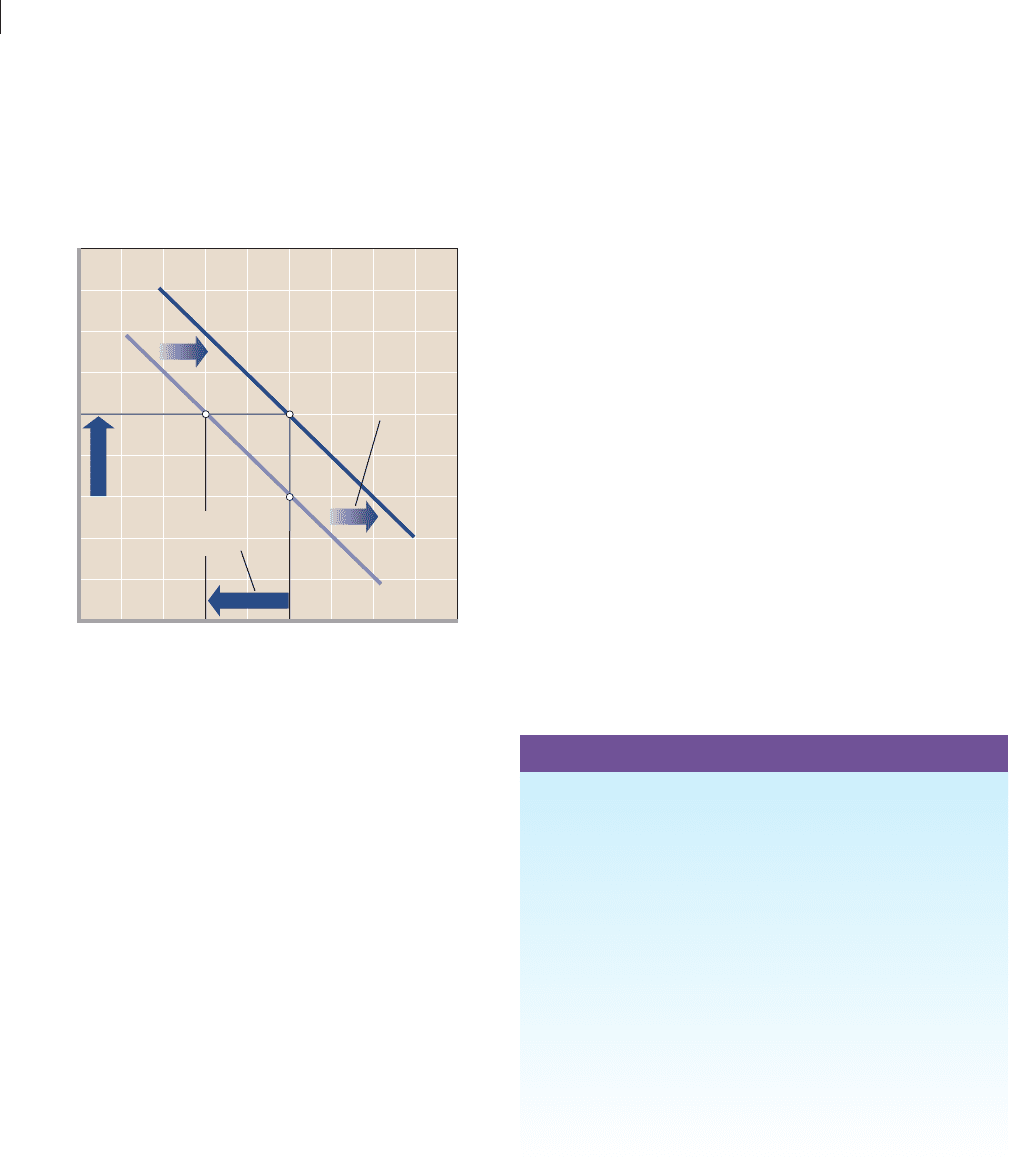
A Graphical Look at Crowding Out We

know from Chapter 8 that the real interest rate is inversely

related to the amount of investment spending. When

graphed, that relationship is shown as a downward-sloping

investment demand curve, such as either ID

or ID

Figure 11.8 . Let’s first consider curve ID

. (Ignore curve

for now.) Suppose that government borrowing

increases the real interest rate from 6 percent to 10 percent.

Investment spending will then fall from $25 billion to

$15 billion, as shown by the economy’s move from a to b .

That is, the financing of the debt will compete with the

financing of private investment projects and crowd out

mcc26632_ch11_208-226.indd 221mcc26632_ch11_208-226.indd 221 8/21/06 4:35:14 PM8/21/06 4:35:14 PM

CONFIRMING PAGES

PART THREE

Macroeconomic Models and Fiscal Policy

222

financing through debt, the stock of public capital passed

on to future generations may be higher than otherwise.

That greater stock of public capital may offset the di-

minished stock of private capital resulting from the

crowding-out effect, leaving overall production capacity

unimpaired.

So-called public-private complementarities are a

second factor that could reduce the crowding out effect.

Some public and private investments are complementary.

Thus, the public investment financed through the debt

could spur some private-sector investment by increasing

its expected rate of return. For example, a Federal

building in a city may encourage private investment in

the form of nearby office buildings, shops, and restaurants.

Through its complementary effect, the spending on

public capital may shift the private investment demand

curve to the right, as from ID

to ID

in Figure 11.8 . Even

though the government borrowing boosts the interest

rate from 6 percent to 10 percent, total private investment

need not fall. In the case shown as the move from a to c in

Figure 11.8 , it remains at $25 billion. Of course, the

increase in investment demand might be smaller than

that shown. If it were smaller, the crowding-out effect

would not be fully offset. But the point is that an increase

in private investment demand may counter the decline in

investment that would otherwise result from the higher

interest rate. (Key Question 13)

QUICK REVIEW 11.3

• The U.S. public debt—nearly $8 trillion in 2005—is

essentially the total accumulation of Federal budget deficits

minus surpluses over time; about 25 percent of the public

debt is held by foreigners.

• As a percentage of GDP, the portion of the debt held by the

public is lower today than it was in the mid-1990s and is in

the middle range of such debts among major industrial

nations.

• The Federal government is in no danger of going bankrupt

because it needs only to refinance (not retire) the public

debt and it can raise revenues, if needed, through higher

taxes.

• The borrowing and interest payments associated with the

public debt may (a) increase income inequality, (b) require

higher taxes, which may dampen incentives, and (c) impede

the growth of the nation’s stock of capital through crowding

out of private investment.

$10 billion of private investment. So the stock of private

capital handed down to future generations will be

$10 billion less than it would have been without the need

to finance the public debt.

Public Investments and Public-Private

Complementarities

But even with crowding

out, two factors could partly or fully offset the net eco-

nomic burden shifted to future generations. First, just as

private goods may involve either consumption or invest-

ment, so it is with public goods. Part of the government

spending enabled by the public debt is for public invest-

ment outlays (for example, highways, mass transit sys-

tems, and electric power facilities) and “human capital”

(for example, investments in education, job training, and

health). Like private expenditures on machinery and

equipment, those public investments increase the

economy’s future production capacity. Because of the

FIGURE 11.8 The investment demand curve and the

crowding-out effect. If the investment demand curve ( ID

) is fixed,

the increase in the interest rate from 6 percent to 10 percent caused by

financing a large public debt will move the economy from a to b and crowd

out $10 billion of private investment and decrease the size of the capital

stock inherited by future generations. However, if the public goods enabled

by the debt improve the investment prospects of businesses, the private

investment demand curve will shift rightward, as from ID

to ID

. That shift

may offset the crowding-out effect wholly or in part. In this case, it moves

the economy from a to c.

Increase in

investment

demand

Crowding-out

effect

Real interest rate (percent)

10 15 20 25 30 35 40

Investment (billions of dollars)

mcc26632_ch11_208-226.indd 222mcc26632_ch11_208-226.indd 222 8/21/06 4:35:15 PM8/21/06 4:35:15 PM

CONFIRMING PAGES