Lima J.J.Pedroso, de (ed.). Nuclear Medicine Physics

Подождите немного. Документ загружается.

218 Nuclear Medicine Physics

to correct the SPECT data. This can be done either when the activity distribu-

tion is analytically reconstructed, in which case the correction is implemented

in a preprocessing procedure before the reconstruction [9–12], or when the

reconstruction is iterative, for which the correction is incorporated in the iter-

ative process [13,14]. The attenuation map can not only be estimated with a

transmission measurement using the SPECT scanner itself [5], as noted later,

but it can also be based on pure morphologic images obtained with other

methods (CT, MRI), in which attenuation coefﬁcients are attributed to the dif-

ferent anatomical regions according to literature values for the different types

of tissue [15,16], or even by anatomical information gathered using scattered

radiation [17,18].

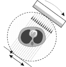
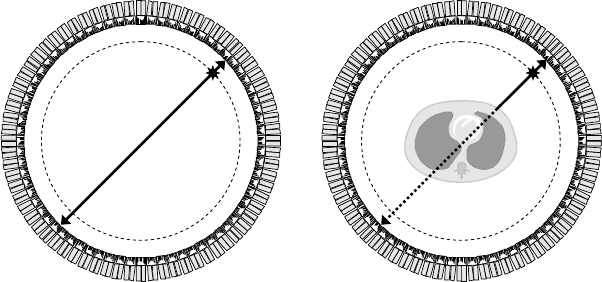
6.2.2.1.2 Transmission Measurement

A transmission measurement consists of determining the fraction of photons

that is transmitted throughout the patient in all the directions deﬁned by

the projection planes. Some SPECT cameras incorporate a CT scanner that

performs this task, but the transmission measurement can also be obtained

using the gamma heads of the SPECT system and an external collimated γ

emitting source, which is rotated around the patient (Figure 6.2).

The γ source may be point-like, linear or planar, but the collimator must

be chosen to suit the type of source used; the most popular combination is a

sweeping linear source with a parallel collimator. The radioactive isotope for

the source has to be long-lived to be of practical use and produce γ photons

with energy near to that emitted by the SPECT marker, so that the attenua-

tion coefﬁcients are approximately the same. When the marker is

99m

Tc, which

emits 140 keV photons, it is customary to use a

153

Gd source for the transmis-

sion measurement, as it produces 100 keV photons and has a half-life of 242

days. The attenuation measurement can be carried out at the same time as or

after the SPECT emission measurement; the ﬁrst mode requires a coincidence

153

FIGURE 6.2

Layout of a transmission measurement, performed with the SPECT system’s detector heads and

an external collimated radioactive source, moved along the projection plane and around the

patient.

Imaging Methodologies 219

system between the transmission source and the illuminated collimators of

the detector head at each instant, but it offers faster exams, thereby reducing

the amount of motion artifacts in the data.

The transmission measurement builds parallel projections of the attenua-

tion map, as the quotient between the number N of transmitted photons and

the number N

emitted by the source in a given direction is related to the

line integral along that direction of the linear attenuation coefﬁcient by the

exponential attenuation law:



direction i



direction i

μ(x, y)dr

direction i

. (6.3)

The nonattenuated measurements N

are obtained in a blank scan, that

is, a measurement in the same acquisition conditions as the transmission

measurement but with no patient. The attenuation map μ(x, y) for each plane

is eventually constructed from the parallel projections of Equation 6.3 using

the ﬁltered backprojection method or any other image reconstruction method

discussed in this chapter.

The use of attenuation correction in the clinical applications of SPECT, for-

merly dismissed due to its complexity, cost, and quality control demands, is

nowadays becoming more widespread owing to the increasing number of

SPECT or CT cameras. The clinical impact of attenuation correction has been

enjoyinggrowingacceptance and is recommended, for example, in cardiology

for myocardial perfusion exams using gated-SPECT [19].

6.2.2.1.3 Correction Methods

Once the attenuation map μ(x, y) is known, the attenuation correction can be

carried out using methods that directly act on the reconstructed image. These

may be analytical methods that correct the SPECT projections before image

reconstruction or iterative methods that correct the projections during image

reconstruction.

The direct method of image correction most often employed in everyday

clinical practice is that proposedby Chang [9], accordingto which the estimate

of the activity distribution f

est

(x, y) in each plane is corrected by

corrected

(x, y) = c(x, y) ×f

est

(x, y), (6.4)

where the correction coefﬁcients c(x, y) are the inverse of the average attenu-

ation calculated over all the emission directions that contain the point (x, y),

that is,

c(x, y) =

2π



−¯μ

(x,y)l

(x,y)

dφ

, (6.5)

220 Nuclear Medicine Physics

with ¯μ

(x, y) being the average linear attenuation coefﬁcient computed from

the point (x, y) up to the border of the patient along direction φ and l

(x, y)

being the thickness of that path. This method, although very easy to imple-

ment, yields poor results when there is a broad activity distribution; In those

cases, it is preferable to apply this type of correction iteratively, successively

improving the correction coefﬁcients by comparing the projections of the

corrected activity distribution, calculated by Equation 6.4, with the original

projections.

Analytical correction methods operate on the acquired projections before

image reconstruction. This type of method is less popular in the clinical envi-

ronment, but its outcome is usually better than the method of Chang. At

present, the main analytical correction method is based on the mathemati-

cal inversion of the attenuated Radon transform proposed by Markoe [10]

from the inversion of the exponential Radon transform previously obtained

by Tretiak and Metz [20]. For each z plane, the SPECT measurements are

the projections of the activity distribution modulated by the attenuation map

according to the exponential attenuation law,

, φ) =

+∞



−∞

f (x, y)e

−

+∞



μ(x



) dy

, (6.6)

where p

, φ) are the parallel projections of f (x, y) attenuated by μ(x, y).

If μ(x, y) is constant, with a value of μ

over the region where f (x, y) is

nonzero,thenthe attenuated projectionscan beconverted into theexponential

projections of f(x, y) with a μ

factor, p

, φ) by

, φ) =

+∞



−∞

f (x, y)e

= e

d(x

,φ)

, φ). (6.7)

In this equation, the function d(x

, φ) is given by

d(x

, φ) = μ

min

, φ) +

+∞



min

,φ)

μ(x, y) dy

, (6.8)

whose value can be computed if we know the attenuation map μ(x, y) and the

lower boundary y

min

, φ) of the region where f (x, y) is nonzero, expressed

in the OX

reference frame ﬁxed to the detection heads (see Section 5.3.1.3,

Figure 5.27). The value of μ

is also obtained from the attenuation map, cor-

responding to the average value of μ(x, y) where f (x, y) is nonzero. It should

be noted that assuming that the linear attenuation coefﬁcient is constant

where the activity is nonzero is generally a good approximation, because the

radiotracer usually concentrates in a single type of tissue. The exponential

Imaging Methodologies 221

projections of f (x, y) are ﬁnally converted into nonattenuated projections

p(x

, φ) by a translation in Fourier space given by the relation

{p}(ν

, φ) = F

}

⎛

⎝





2φ



, φ +i sinh

−1

⎞

⎠

, (6.9)

where F

is the one-dimensional Fourier transform with regard to x

of the

operand function. With this equation, and executing a Fourier series expan-

sion to compute the complex angles which are the arguments of the Fourier

transform of p

, φ), we obtain the nonattenuated projections that will be

used in the analytical image reconstruction process.

For the iterative correction methods, the attenuation correction is included

in the iterative image reconstruction process itself. This is currently the most

widely used correction method in clinical practice today [21,22], operating

at the level of constructing the activity projections too. In each iteration, the

attenuation map is employed via Equation 6.6 to calculate the attenuated

projections from the activity distribution estimate proposed in that iteration.

Those attenuated projections are compared with the measured projections,

and the estimated activity distribution is updated according to the result of

that comparison. Image reconstruction, thus, follows the usual course of iter-

ative methods, with the single difference being in the model of formation of

the parallel projections from the activity distribution estimates.

6.2.2.1.4 Correction of Scattered Radiation

Correcting scattered radiation in SPECT involves determining the number of

γ photons detected along each direction in space that has not suffered any

Compton scattering interaction. The products of this type of interaction, as

referred to in Chapter 5 (see Figure 5.6), are one electron and one γ photon

that share the energy of the incident photon. The scattered photon is emitted

along a direction θ relative to the incident photon and carries an energy given

by Equation 5.5.

The energy E



carried by the scattered photon is always smaller than the

energy of the incident photon, and this fact can be used to distinguish photons

that have undergone Compton scattering from those that have not, by simply

measuring the energy of the detected photons. The correction of scattered

radiation must be performed before the attenuation correction, so that the

latter will solely operate on the nonscattered photons, which are the only

ones whose direction bears a causality relation with their emission points.

Executing the energy discrimination of the detected photons is, therefore,

the simplest way of estimating the number S of scattered photons, a value

that can then be subtracted from the total number of detected photons C to

obtain the number of nonscattered photons T in each direction of the parallel

projections:

T = C −S. (6.10)

222 Nuclear Medicine Physics

Number of photon

counts

Energy

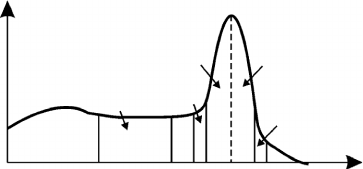
FIGURE 6.3

Typical energy histogram of the photons detected in a channel of a SPECT scanner and corre-

sponding division in the energy windows normally used to perform the correction of scattered

radiation (W1–W5). The number of windows actually employed depends on the method chosen

for the correction.

There are several empirical methods to estimate the value of S in a given

direction from the energy histogram of the detected photons, based on count-

ing the number of photons inside different energy windows around the

photopeak (Figure 6.3) [23–25]. The actual estimate of S is calculated by taking

into account the total number of counts in each energy window, the width of

the windows, and other simple parameters obtained from empirical studies

of scattered radiation in SPECT.

Scatteredradiation can alternatively be corrected using methods that model

the existence of Compton scattering in the body of the patient. One of the

simplest consists of using attenuation coefﬁcients that are lower than those

obtained in the transmission measurement [26]. The underassessment of the

attenuation map takes into account the increase of the number of detected

photons due to the presence of scattered radiation. The degree of underassess-

ment that should be used depends, however, on the nature of each tissue and

has to be known beforehand for all the structures present in the activity dis-

tribution. One other, rather more sophisticated, correction model is based on

computing the scattered radiation map of the patient from his or her anatom-

ical features [27,28]. This map is constructed using the attenuation map in

conjunction with the knowledge of the type of tissue existing in each point

of that map, to estimate the probability of Compton scattering occurring in

that point.

6.2.2.1.5 Spatial Resolution Correction

In addition to the physical effects that affect SPECT measurements, partic-

ularly attenuation and scattered radiation, certain instrumental factors also

inﬂuence image formation. The strong dependence of the spatial resolution

of a SPECT scanner on the distance to the detector heads, due to the use of

physical collimators, is the most important of those factors. Associated with

that dependence, moreover, is the fact that the point spread function, that is,

Imaging Methodologies 223

the function which quantiﬁes the spatial resolution of the tomograph [29],

has a ﬁnite width, giving rise to what is known as the partial volume effect.

This effect mostly inﬂuences the observation of small structures, with dimen-

sions of less than 2 to 3 times the spatial resolution of the camera, and it is

expressed in an undervaluation of the activity in high-activity structures rel-

ative to the surrounding tissues as well as in an overvaluation of those which

have low activity [30]. The ﬁnite width of the point spread function producesa

smoothing of the boundaries between adjacent tissues with different activity

concentrations in the ﬁnal image, blurring all the abrupt transitions of activity

(Figure 6.4). In other words, the high spatial frequencies found in the activity

distribution are ﬁltered by the point spread function of the system. The spa-

tial resolution correction is only carried out after the scattered radiation and

attenuation corrections, although it is seldom used in clinical practice.

The correction methods for the partial volume effect in SPECT, which

include the dependence of the spatial resolution on the distance to the detec-

tor heads, can be grouped in three categories: deconvolution methods [31,32],

methods that model the effect of spatial resolution during iterative image

reconstruction [33–35], and methods that use morphological information

independently obtained from the SPECT measurement [36].

Inthe ﬁrstcategory, the measuredprojectionsarecorrectedjust beforeimage

reconstruction. The correction is based on the fact that the image produced

in a tomograph is the convolution of the activity distribution with the point

spreadfunction of the tomograph. For each reconstructionplane, this function

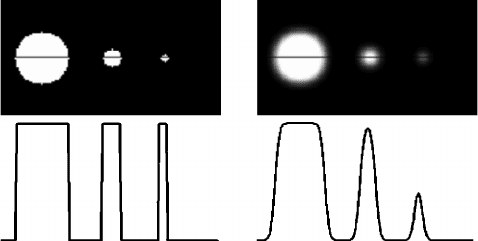
Original Image produced by the tomograph

FIGURE 6.4

The partial volume effect. (left) Activity distribution in an ideal tomograph capable of exactly

reproducing the object in the ﬁeld of view and (right) corresponding image in a tomograph with

ﬁnite spatial resolution, equal to the dimension of the smallest structure in the image. The other

structures have dimensions of 2, 3, and 4 times the spatial resolution. Below the two top images,

the activity measured along the dashed line is also shown. In the right image, the abrupt activity

transitions have been smoothed by the tomograph; the image produced is the convolution of

the activity distribution with the point spread function of the system. The error in the activity

recorded in small structures can be quite signiﬁcant, as observed in the rightmost structure.

224 Nuclear Medicine Physics

is given to a good approximation by a Gaussian function of the type

PSF(x, y) = e

−

(x−x

)

+(y−y

)

(6.11)

in each point (x

, y

) of that plane, with a width σ(x

, y

) that changes from

point-to-point and which may be experimentally determined during the char-

acterization routines of the tomograph. Knowing the point spread function, it

becomes possible to correct the measured projections using the mathematical

deconvolution of the data, which reduces simply to a division in the Fourier

space.

In the second group, the point spread function is also used to convolute the

estimate of the activity distribution in each iteration of the image reconstruc-

tion process, before computing the parallel projections corresponding to that

estimate. The comparison of the convoluted estimated projections with the

acquired projections takes into account the fact that the acquired projections

are subject to the partial volume effect.

Finally, the third category includes recently proposed correction methods

which adjust the activity distribution measured by the SPECT camera to the

morphology of the tissues underlying that distribution. The adjustment is

performed by forcing the activity in a given region to be conﬁned to the tis-

sues where the radiotracer is located; in particular, the activity in supposedly

nonactive tissues is transferred to the nearest tissues capable of ﬁxing the

radiotracer. These methods imply the use of images separately obtained with

morphological techniques (CT, MRI) from the SPECT measurement.

6.2.2.2 PET

6.2.2.2.1 Attenuation Correction in PET

Just as in SPECT, PET measurements are liable to be affected by attenuation,

which occurs when the two photons of an annihilation pair traverse the path

leading from the annihilation site to the crystals where they will be detected.

This means that for a given LOR, the number of photon pairs hitting the two

detectors is smaller than the number of photon pairs emitted along that LOR.

There are, however, two major differences between PET and SPECT with

regard to attenuation. First, attenuation is more pronounced in PET, as both

photons have to escape the patient’s body without interacting for a coinci-

dence to be detected. The fraction of decays in the patient that gives rise

to a counting event (a coincidence in the case of PET and a single photon in

SPECT) along a given direction is, therefore, considerably smaller in PET than

in SPECT.

Thesecond differencelies inthe factthat attenuationinPET doesnot depend

on the position of the emission point, in marked contrast to what happens

in SPECT. This is easily seen if we take a simple situation consisting of a

point source located inside a uniform body with a constant linear attenuation

Imaging Methodologies 225

coefﬁcient; for that object, the coincidence count rate recorded in an line of

response (LOR) passing through the source, A

, is given as a function of the

activity of the source in that direction by

, φ) = A



−μy

×e

−μy



= Ae

−μ(y

)

= Ae

−μl(x

,φ)

, (6.12)

as the sum of the distances y

and y

traveled by the two photons of one

annihilation pair inside the body is the total thickness l(x

, φ) of that body

along the direction of the LOR. The factor e

−μl(x

,φ)

depends on the full thick-

ness traveled by the photon pair and not on the speciﬁc location of the source

along the LOR. This is why estimating the attenuation factors is very sim-

ple and precise in PET compared with the attenuation correction methods of

SPECT.

The distribution of attenuation factors in the object is obtained using trans-

mission measurements that can be carried out with multienergy x-ray sources

in PET or CT systems (described in the next section) or in PET systems with

single-energysources,which can be either positronor gamma photon sources;

Figure 6.5 shows these three possibilities. For the latter, the most common

sources used are

Ge, a positron emitter, or

137

Cs, a gamma emitter that pro-

duces single gamma photons with an energy of 662 keV [37,38]. The number

of photons transmitted in each LOR, N, is given as a function of the number

of photon pairs emitted in that LOR, N

, by the exponential attenuation law

N = N

−



μ(y

) dy

, (6.13)

where the nonattenuated measurements are collected in a blank scan carried

out in exactly the same conditions as the transmission measurement but hav-

ing no patient. To compute the correction sinograms having (the inverse of)

the attenuation factors e

−



μ(y

) dy

, we divide the blank scan sinograms by

the sinograms of the transmission measurement. The attenuation correction

511

keV

(a) (b) (c)

keV

120

662

keV

137

FIGURE 6.5

Diagramshowing thethreeways ofmeasuring attenuationfactors ofa patient,using (a)a positron

emitter; (b) a gamma emitter; (c) and an x-ray source. The measured attenuation factors depend

on the layout of organs and tissues in the patient and on the energy of the radiation produced

by the source.

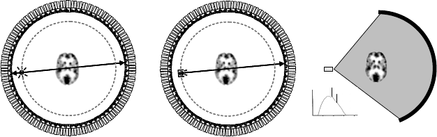
226 Nuclear Medicine Physics

Rotating

source

Blank scan

Transmission scan

Rotating

source

FIGURE 6.6

Representation of the attenuation correction in PET using a transmission measurement with a

rotating radioactive source. (Left) blank scan, that is, an acquisition without having the patient

in the scanner’s FOV; (right) transmission measurement with the patient in the FOV.

is eventually performed by multiplying point by point the sinograms of the

PET acquisition with the sinograms of the attenuation factors [37–39].

The comparison of the transmission measurement data collected with and

without the patient in the FOV of the camera, thus, provides a direct estimate

of the attenuation in each LOR. The quotient sinograms obtained are enough

to perform the correction, although there are situations when it is necessary

to actually know the attenuation map, implying the reconstruction of the

transmission data. Once this image is computed, the data can be segmented to

suppress noise, for example, and only afterward it should be used to generate

the attenuation correction factors (Figure 6.6).

6.2.2.2.2 Attenuation Correction in PET or CT

6.2.2.2.2.1 Attenuation Based on Polyenergetic Transmission (x-rays) In com-

puted axial tomography (CAT or CT) scans, the values proportional to the

linear attenuation in each point of the slice under consideration are stored

in digital form in the computer memory, starting from the smaller to larger

values, addressed in well-determined positions. The wide variety of attenu-

ation coefﬁcient values that can occur in CT images can be estimated from

Figure 6.7 [40].

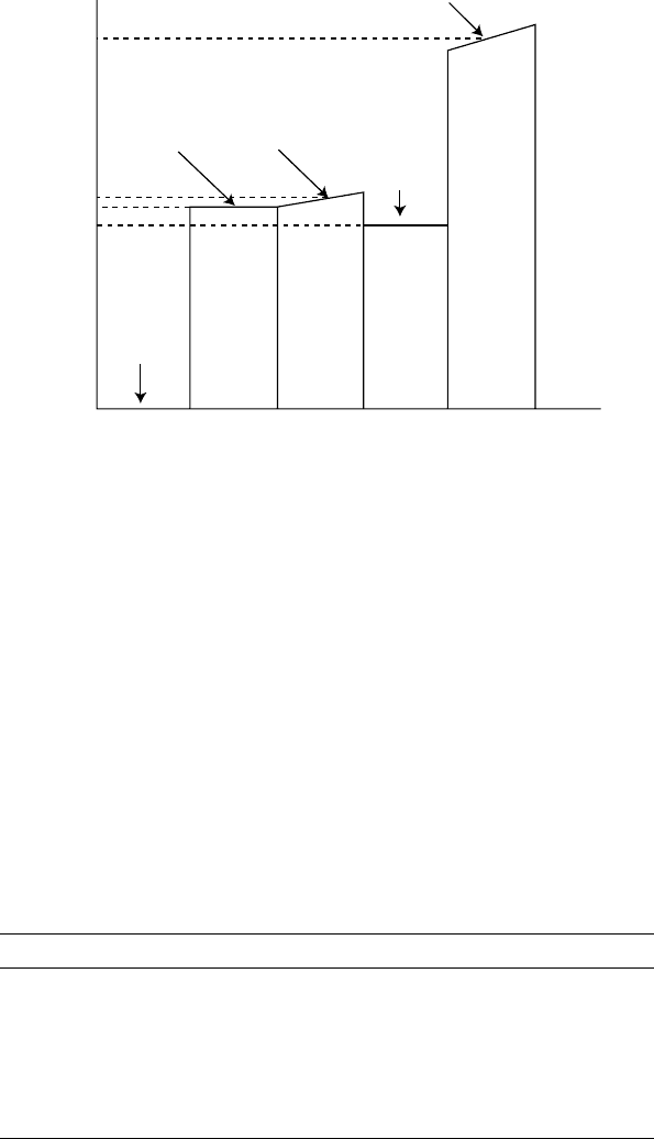
The ﬁgure shows the attenuation coefﬁcient values from media that absorb

x-rays in the human body, with the values given as percentages. Water is

attributed the value 0, and air corresponds to the value −100. It can be seen

that fat tissue absorbs 10% less than water, soft tissue can absorb up to 4%

more than water, and bone can exceed 100% absorption also relative to water.

The attenuation coefﬁcients obtained with CT scans are not usually expressed

Imaging Methodologies 227

100

–10

–100

Air

Water

Soft tissue

Fat

Bone

FIGURE 6.7

Attenuation coefﬁcients for several human components of biological relevance, given in percent-

age with water and air having values of 0 and −100%, respectively. (From De Lima, J. J. P. Eur. J.

Phys., 19:485–497, 1998.)

in percentages but in Hounsﬁeld units (HU). On this scale, named after its

inventor, air corresponds to −1000 HU and water to 0 HU.

Table 6.1 gives various HU values and their corresponding linear attenu-

ation coefﬁcients, obtained for two peak voltages commonly used in clinical

practice.

In modern PET or CT scanners, the attenuation maps used to compute the

attenuation of 511 keV radiation detected with the PET system are generated

from the CT scan of the patient, performed either before or straight after

the PET scan. The CAT scan data are given in HU, as mentioned. These HU

values cannot be directly used to correct the attenuation of the emission data,

TABLE 6.1

Hounsﬁeld Units (HU) and Linear Attenuation Coefﬁcients for Two Peak

Voltages and Different Materials and Tissues

84 kVp μ (cm

−1

) 12 kVp μ (cm

−1

)

Air −1000 0.0003 0.0002

Water 0 0.180 0.160

Fat −100 0.162 0.144

Blood 40 0.182 0.163

Gray matter 43 0.184 0.163

White matter 6 0.187 0.166

Source: From De Lima, J. J. P. Eur. J. Phys., 19:485–497, 1998. With permission.