Layer E., Tomczyk K. (editors) Measurements, Modelling and Simulation of Dynamic Systems
Подождите немного. Документ загружается.


4.9 Levenberg-Marquardt Algorithm 111
4.9 Levenberg-Marquardt Algorithm
In this subchapter, we will present Levenberg-Marquardt optimization algorithm
and discuss the potential of using it for identification. Application of this
algorithm has many advantages in comparison with other optimization methods. It
combines the steepest descent method with Gauss-Newton method, and operates
correctly in search for parameters both far from and close to the optimum one. In
the first situation the algorithm of the linear model of steepest descent is used, and
in the second one-the squared convergence. The fast convergence is the additional
advantage of the algorithm.
Levenberg-Marquardt algorithm is the iterative method, in which the vector of
unknown parameters, for the step
,1+k is determined by the equation
),(),(]),(),([
1
1
xxxx
kk
T
kkk
T
T
kk
zzJIzJzJzz
εμ
−
+
+=
(4.118)
with the approximation error
∑
=
=
n
i
ikk
xx
1
2
),(),( zz
εε
(4.119)
where
⎥
⎥
⎥
⎥
⎦
⎤
⎢
⎢
⎢
⎢
⎣
⎡
−
−
−
=
),(
.
),(
),(
),(
22
11
xzy
xzy
xzy
x
nn
k
φ
φ
φ
ε
z
(4.120)
⎥
⎥
⎥
⎥
⎥
⎥
⎥
⎥
⎦
⎤
⎢
⎢
⎢
⎢
⎢
⎢
⎢
⎢
⎣
⎡
∂
∂
∂
∂
∂
∂
∂
∂
∂
∂
∂
∂
∂
∂
∂
∂
∂
∂
=
m
nknknk
m
kkk
m
kkk
k
z
x
z
x
z
x
z
x
z
x
z
x
z
x
z
x
z
x
x
),(
.
),(),(
....
),(
.
),(),(
),(
.
),(),(
),(
21
2
2
2
1
2
1
2
1
1
1
zzz
zzz
zzz
zJ
εεε
εεε
εεε
(4.121)
The notations in )121.4()118.4( − are as follows: ,...,,2,1 pk = −p a number
of iteration loops, J
nxm
−),( x
k
z Jacobian matrix, I
mxm
unit− matrix, −
k
μ
scalar,
−= ]...,,,[
21 n
xxxx vector of input parameters, −= ]...,,,[
21 n
yyyy vector of
output parameters, −= ),(φ xzy
predicted model, −= ]...,,,[
21 m
zzzz unknown
parameters.

112 4 Model Development
Levenberg-Marquardt algorithm is used for computation in two steps:
Step 1
the initial values of the vector
k
z
assume− the initial value of the coefficient
k
μ
(e.g.
k
μ
= 0.1)
solve− the matrix equations (4.120) and (4.121)
calculate− the value of error (4.119)
determine− the parameters of the vector ,
1+k
z according to (4.118).
Step 2 and further steps
update− the values of the parameter vector for the model y
solve− the matrix equations (4.120), (4.121) and (4.118)
calculate− the value of error (4.119)
compare− the values of error (4.119) for the step k and the step .1−k
If the result is ),,(),(
1
xx
kk −
≥ zz
εε
multiply
k
μ by the specified value ℜ∈
λ
(e.g. 10=
λ
) and return to the step 2. If the result is ),(),(
1
xx
kk −
< zz
εε
divide
k
μ
by the value
λ
and return to the step 1.
If in the consecutive steps a decreasing in the value of error (4.119) is very
small and insignificant, we then finish the iteration process. We fix 0=
k
μ
and
determine the final result for the parameter vector.
If the value of coefficient
k
μ
is high, it means that the solution is not
satisfactory. The values of the parameter vector z are not optimum ones, and the
value of error (4.119) is not at minimum level. At this point it can be assumed
IzJzJ
kkk
T
xx
μ
<<),(),(
(4.122)
and this leads to the steepest descent method, for which we have
),(),(
1
1
xx
kk
T
k
T
kk
zzJzz
ε
μ
−=
+
(4.123)
If the value of the coefficient
k
μ
is small, it means that the values of the vector
z parameters are close to the optimum solution,
then
IzJzJ
kkk
T
xx
μ
>>),(),(
(4.124)
and Levenberg-Marquardt algorithm is reduced to Gauss-Newton method
),(),()],(),([
1
1
xxxx
kk
T
kk
T
T
kk
zzJzJzJzz
ε
−
+
−=
(4.125)
The selection of the coefficient values
k
μ
and
λ
depends on assumed programs
and selected software.

4.9 Levenberg-Marquardt Algorithm 113
4.9.1 Implementing Levenberg-Marquardt Algorithm Using
LabVIEW
It is convenient to deploy Levenberg-Marquardt algorithm with LabVIEW
software. Fig. 4.17. presents the block diagram of the measuring system for
determining any characteristics of investigated object in this program
Measurement data given by vectors x and y are sent to the measuring system
through its analogue output and are recorded into the text files (Write to
Measurement File1 and Write to Measurement File2, respectively). These data are
next in the Curve Fitting block approximated by means of Levenberg-Marquardt
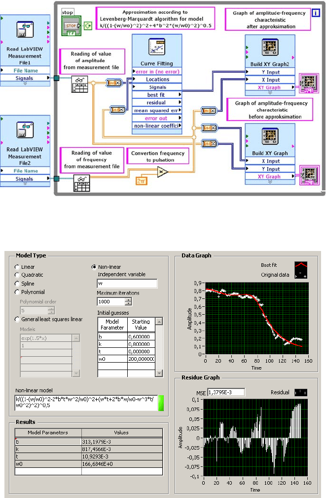
algorithm. Fig. 4.18. presents the diagram of the general data approximation
system, while Fig. 4.19. illustrates the Curve Fitting approximation block adapted
for the exemplary approximation of frequency characteristic of the third-order
system (in Non-linear model window).
Fig. 4.17 Diagram of measuring system for determination of frequency characteristics
The approximation process is carried out for the initial value of parameters
(Initial guesses) and number of iteration (Maximum iterations). Windows Results
presents the value of calculated parameters and the value of mean square error
(MSE).
114 4 Model Development
Fig. 4.18 Diagram of measuring system for approximation of frequency characteristics in
LabVIEW
Fig. 4.19 Curve Fitting block (Fig. 4.18) for approximation of third-order system
4.10 Black-Box Identification 115
4.10 Black-Box Identification
In the black-box identification, the experiment is carried out using discrete
measurement data. From among preset parametric models, being a good match for
these data, the desired model structure is selected. The discrete model of the
identified object, in the form of the transfer function, is taken under consideration
n
m
m
zzaa
zbzbb
zK
−−
−−
+++
+++
=
...
...
)(
1
10
1
10
(4.126)
or equivalent one
][)(][)(
11
kzkz uByA
−−
=
(4.127)
where
n
zzaaz
−−−
+++= ...)(
1
10
1
A
(4.128)
m
m
zbzbbz
−−−
+++= ...)(
1
10
1
B
(4.129)
Nnnkk
z
n
∈−=
−
,][][ xx
(4.130)
for which a white noise ][k
e is added and the parametric model of ARX type
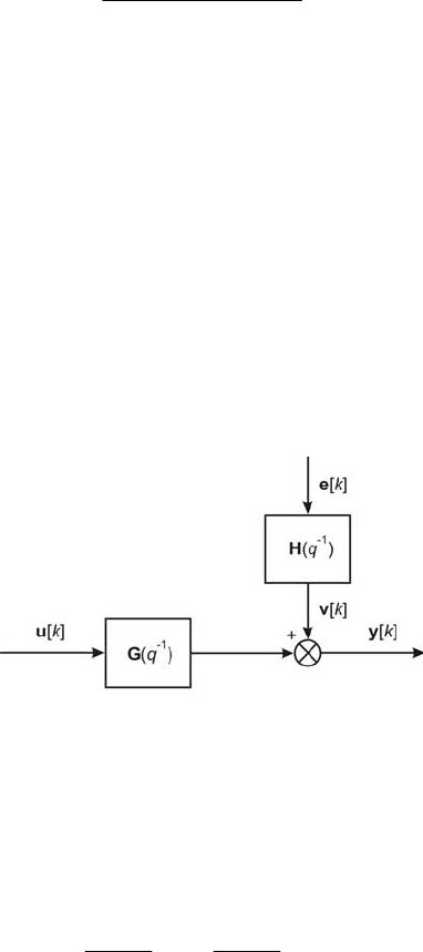
(Auto Regressive with eXogenous input) is formulated.
Fig. 4.20 ARX model, −)(tv noise
Now we have
][][)(][)(
11
kkzkz euByA +=
−−
(4.131)
and from it
][
)(
1
][
)(
)(
][
11
1
k
z
k
z
z
k
e
A
u
A
B
y
−−
−
+=
(4.132)

116 4 Model Development
where in )132.4()127.4( − ],[ku ][ky are the input and output signals at the
discrete time
,k ][kx is any measurement data in k and
1−
z is delayed at one.
Denoting
)(
1
)(
1
1
−
−
=
z
z
A
H
(4.133)
we finally have
][)(][)(][
11
kzkzk eHuKy
−−
+=
(4.134)
Eq. (4.134) describes the ARX model shown in Fig. 4.20. Identification of the
ARX model is based on the following assumptions
the− object )(
1−
zK is asymptotically stable
the− filter )(
1−
zH is linear, asymptotically stable, minimum-phase and invertible
the− input signal variation ][ku is sufficiently large
and leads to a simultaneous solution of two following tasks
tionidentifica− of the object, of which the transfer function is )(
1−
zK
tionidentifica− of the filter ).(
1−
qH
Let us present the equation (4.132) as follows
][][][ kkk
eΦzy +=
(4.135)
where
]][...,],[],1[...,],1[[][ mkkkkk −−−−−=
uuyyz
(4.136)
]...,,,1,...,,[
010 mn
T
bbaa
−
=Φ
(4.137)
Let us also denote by p the number of activating signals. Then Eq. (4.135) takes
the final form
⎥
⎥
⎥
⎦
⎤
⎢
⎢
⎢
⎣
⎡
+
⎥
⎥
⎥
⎦
⎤
⎢
⎢
⎢
⎣
⎡
=
⎥
⎥
⎥
⎦
⎤
⎢
⎢
⎢
⎣
⎡
−−−
][
.
][
][
.
][
][
.
][
1
0
1
0
1
0
ke
ke
kz
kz
ky
ky
ppp
Φ
(4.138)
As the result the identification task is reduced to the determination of the estimates
of model parameters
)(
][],[,, kkmn yuΦ Θ=
∧
(4.139)

4.10 Black-Box Identification 117
Apart of the ARX model, there are also other structures applied quite often:
AR−
model described by the equation
0][)(
1
=
−
kz yA
(4.140)
ARMAX−
model described by
][)(][)(][)(
111
kznkkzkz eCuByA
−−−
+−=
(4.141)
−
Box-Jenkins model
][
)(
)(
][
)(
)(
][
1
1
1
1
ke
z
z
k
z
z
k
−
−
−
−
+−=
D
C
u
F
B
y
δ
(4.142)
where
...)(
1
10
1
++=
−−
zcczC
(4.143)
...)(
1
10
1
++=
−−
zddzD
(4.144)
...)(
1
10
1
++=
−−
zffzF
(4.145)
and
δ
is a number of delaying steps between the input and output.
4.11 Implementing Black-Box Identification Using MATLAB
One of the models listed in System Identification Toolbox library of MATLAB
software is the model
[] [] []
k
q
q
nkk
q
q
kq e
D
C
u
F
B
yA
)(
)(
)(
)(
)(
1
1
1
1
1
−
−
−
−
−
+−=
(4.146)
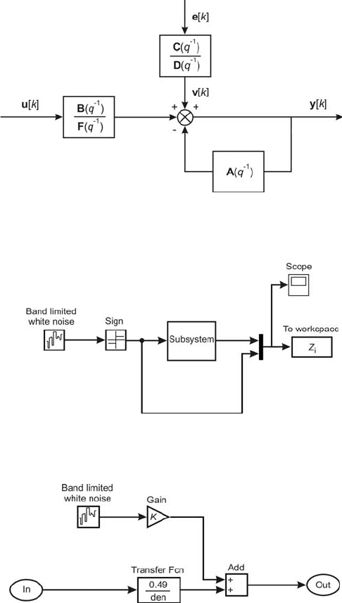
Its structure is shown in Fig. 4.21. The models (4.132) and )142.4()140.4( − are
the special cases of (4.146).
We apply the black-box method to the ARX model and the virtual object
defined by the discrete Laplace transform. Using MATLAB, the identification
experiment is carried out in the following steps:
In the first step the measuring system in Simulink program is set −up Fig. 4.22.
Its Subsystem block is shown in Fig. 4.23. The Sign block executes )(xsigny =
relation while Band-Limited White Noise is the white noise generator. Generation
method of this signal is described in the menu under Seed. The block Transfer Fcn
represents the digital transfer function of identified object.
118 4 Model Development
Fig. 4.21 Model structure applied in Identification Toolbox library
Fig. 4.22 Measuring system in Simulink program
Fig. 4.23 Internal structure of Subsystem block
In the second step by means of To Workspace block, measured data are
transferred and read into MATLAB working environment, and recorded as the Z
1
matrix. The vectors ][ku and ][ky are used during identification process
4.10 Black-Box Identification 119
Z
1
=
⎥
⎥
⎥
⎦
⎤
⎢
⎢
⎢
⎣
⎡
][][
..
[[][
11
kuky
kuky
mm
(4.147)
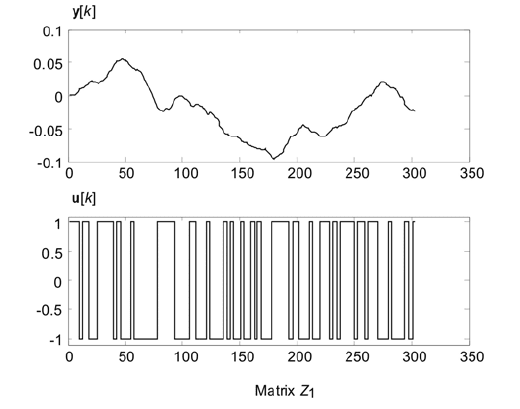
As an example, obtained through the command
>>
idplot(Z
1
)
for den = [1 4.2 0.49] and Seed = [1 2 3 1 2], data of the first measured series
of 300 samples, are shown in Fig. 4.24.
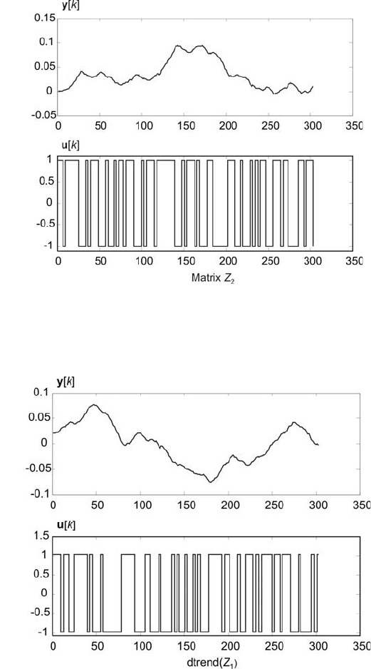
Fig. 4.24 Examples of data from second measuring series
The second series of measurements is used for a verification of the given
model, and is recorded in
Z
2
matrix. However, the setup of Seed block must be
changed before starting these measurements. Examples of measurement results
Z
2
for Seed = [4 3 4 1 2] are shown in Fig. 4.25.
In the third step errors generated by noise and random trends are removed.
Completing this task is possible using the
trend function, for which
>>
Z
11
= dtrend(Z
1
)
and
>>
Z
22
= dtrend(Z
2
)
are corresponding matrices of processed data contained in Z
1
and Z
2
. The input
and output functions, obtained through the applied
dtrend function, are shown in
Fig. 4.26 and Fig. 4.27.
120 4 Model Development
Fig. 4.25
Examples of data from second measured series
Fig. 4.26 Input and output functions obtained through dtrend(Z
1
)
