Layer E., Tomczyk K. (editors) Measurements, Modelling and Simulation of Dynamic Systems
Подождите немного. Документ загружается.

4.3 Legendre Polynomials 91
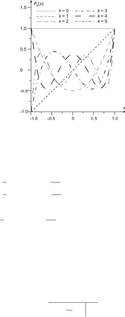
Fig. 4.5 The first five Legendre polynomials
After substituting Eq. (4.25) into Eq. (4.24) and taking (4.26) into account, the
system of equations (4.29) can be obtained, where the vector of coefficients
a presents the solution
[]
[]
[]
⎥
⎥
⎥
⎥
⎥
⎥
⎦
⎤
⎢
⎢
⎢
⎢
⎢
⎢
⎣
⎡
=
⎥
⎥
⎥
⎥
⎥
⎥
⎦
⎤
⎢
⎢
⎢
⎢
⎢
⎢
⎣
⎡
⋅
⎥
⎥
⎥
⎥
⎥
⎥
⎥
⎥
⎦
⎤
⎢
⎢
⎢
⎢
⎢
⎢
⎢
⎢
⎣
⎡
−−−
−
−
−−−
−
−
−−−
−
−
−−
−−−−−−
−−
−−
)(
.
.
)(
)(
.
.
)()2()()22(
1
1
..)13(
2
1
1
......
......
)()2()()22(
1
1
..)13(
2
1
1
)()2()()22(
1
1
..)13(
2
1
1
1
1
0
1
1
0
13120
2
11
13121
2
11
03020
2
00
nn
nnnnnn
nn
nn
xf
xf
xf
a
a
a
xPnxPxn
n
xx
xPnxPxn
n
xx
xPnxPxn
n
xx
(4.29)
Replacing )(xT
k
in (4.16) by )(xP
k
of (4.26) gives
k
xx
kk
k
k
xP
dx
d
xx
xP
xC
=
−
=
)()(
)(
)(
(4.30)
92 4 Model Development
for which the polynomial (4.24) can be presented as
∑
=
−
=
1
0
)()()(
n
k
kk
xCxfxP
(4.31)
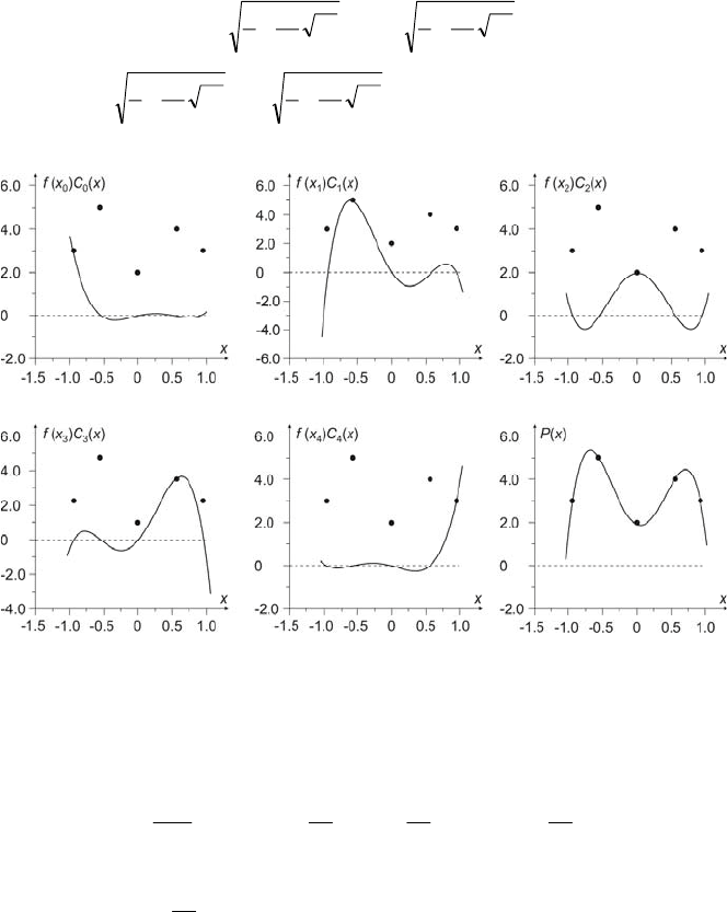
Fig. 4.6 shows the components of polynomial (4.31) for five exemplary measuring
points, which are determined by zeros of the fifth order polynomial and by
measuring data )(
k
xf equal 3, 5, 2, 4 and 3, respectively
⎥
⎥
⎦
⎤
+−
⎢
⎢
⎣
⎡
−−+−=
3,70
63
2
9
5
;4,70
63
2
9
5
;2,0;5,70
63
2
9
5
;3,70
63
2
9
5
)](,[ xfx
Fig. 4.6 Exemplary components of polynomial (4.31)
From (4.20), it can be noticed that shifted Legendre polynomials in the interval
],0[ b are presented by (4.32)
b
x
xP
xP
b
x
Pk
b
x
P
b
x
k
k
xP
kkk
2
1)(
1)(
)
2
1()
2
1()
2
1()12(
1
1
)(
1
0
11
+−=
=
⎥
⎦
⎤
⎢
⎣
⎡
+−−+−+−+
+
=
−+
(4.32)

4.4 Hermite Polynomials 93
A few shifted Legendre polynomials in the interval ],0[ b are given by
9988
77665544
3322
5
776655
443322
4
55443322
3
3322
2
1
0
/2688/12096
/239683/83368/2104045/490324
9/3491830/2748190/11677180/1507)(
3/11203/39209/17360
9/143309/731018/467318/86336/139)(
3/1603/4009/11603/188/169/16)(
/12/18/81)(
/21)(
1)(
bxbx
bxbxbbx
bxbxbxxP
bxbxbx
bxbxbxbxP
bxbxbxbxbxxP
bxbxbxxP
bxxP
xP
+−
+−+−
+−+−=
+−+
−+−+−=
+−+−+−=
−+−=
+−=
=
(4.33)
4.4 Hermite Polynomials
In each measuring point, Hermite polynomials )(xH satisfy the conditions related
to the individual measuring points and to the value of derivatives in these points
)()(),()(
iiii
xf
dx
d
x
dx
dH
xfxH ==
(4.34)
The individual Hermite polynomials can be determined with the use of the
recurrence formula
1,...,2,1,2)(
1)(
)(2)(2)(
1
0
11
−==
=
−=
−+
nkxxH
xH
xkHxxHxH
kkk
(4.35)
Some of the initial Hermite polynomials are as follows
1)(
0
=xH
xxH 2)(
1
=
24)(
2
2
−= xxH
xxxH 128)(
3
3
−=
124816)(
24
4
+−= xxxH
xxxxH 12016032)(
35
5
+−=
(4.36)
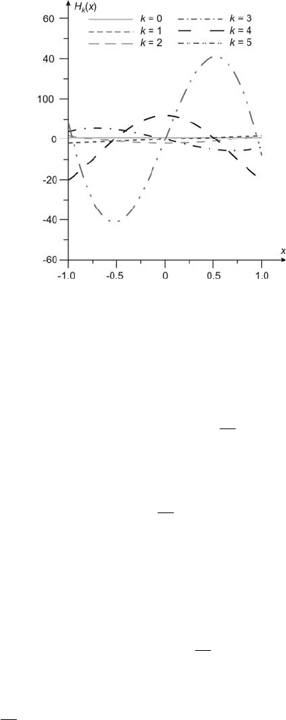
and are shown in Fig. 4.7.
94 4 Model Development
Fig. 4.7 The first six Hermite polynomials
Hermite polynomial )(xH can be defined with a use of the cardinal functions
)(xC
k
(4.8)
)]()()()([)(
1
0
xf
dx
d
xKxfxHxH
n
k
kkk
∑
+=
−
=
(4.37)
where
))(()(
))((21)()(
2
2
kkk
kkkkk
xxxCxK
xxxC
dx
d
xCxH
−=
⎥
⎦
⎤
⎢
⎣
⎡
−−=
(4.38)
It is easy to see that the functions )(
ik
xH and )(
ik
xK fulfill the following
relation
0)(
if0
if1
)( =
⎩
⎨
⎧
≠
=
=
ikik
xH
dx
d
ki
ki
xH
(4.39)
0)(
if0
if1
)( =
⎩
⎨
⎧
≠
=
=
ikik
xK
ki
ki
xK
dx
d
(4.40)
4.5 Cubic Splines 95
Hermite polynomials are orthogonal with the weight function
2
)(
x
exw
−
=
∫
⎩
⎨
⎧
=
≠
=
∞
∞−
−
nmn
nm
dxexHxH
n
x
nm
if!2
if0
)()(
2
π
(4.41)
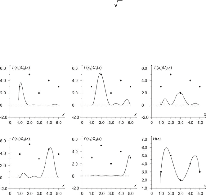
Fig. 4.8 shows the components of polynomial (4.37) for five exemplary measuring
points
]3,5;4,4;2,3;5,2;3,1[)](,[ =xfx and
]7.9;3.3;7.0;7.3;3.12[)( −−−=xf
d
x
d
Fig. 4.8 Exemplary components of polynomial (4.36)
4.5 Cubic Splines
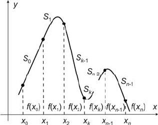
Cubic splines method is based on splitting the given interval into a collection of
subintervals and constructing different approximating polynomials
)(xS
k
at each
subinterval. We use such a cubic polynomial between each successive pair of
points, and the polynomial has the continuous first and second-order derivatives at
these points.
We have three types of cubic splines, and the selection depends on the value of
the second-order derivatives
)(
00
xS
′′
and
)(
nn
xS
′′
at the end-points
0
x
and
.
n
x
96 4 Model Development
1.
The natural spline, for which the second-order derivatives at the end-
points equal zero, i.e.
0)()(
00
=
′′
=
′′
nn
xSxS
2.
The parabolic runout spline, for which the second-order derivatives at the
first and second point are equal, i.e.
0)()(
1100
≠
′′
=
′′
xSxS
. Regarding
the last and one before last point, the second-order derivatives are equal
and different then zero, i.e.
0)()(
1
≠
′′
=
′′
−nn
xSxS
3.
The cubic runout spline, for which the second-order derivatives at the
end-points are different then zero and fulfill the following conditions
)()(2)(
221100
xSxSxS
′′
−
′′
=
′′
and ).()(2)(
2211 −−−−
′′
−
′′
=
′′
nnnnn
xSxSxS
The general form of cubic polynomial is as follows
32
)()()()(
kkkkkkkk
xxdxxcxxbaxS −+−+−+=
(4.42)
For each measuring points
k
x we have
1...,,1,0),()( −== nkxfxS
kkk
(4.43)
where n is the number of measuring points
Fig. 4.9 Cubic splines
For each point, except the first and the last point, the particular polynomials fulfill
the following conditions
)()(
1 kkkk
xSxS
−
=
(4.44)
)()(
1 kkkk
xSxS
−
′
=
′
(4.45)
)()(
1 kkkk
xSxS
−
′′
=
′′
(4.46)

4.5 Cubic Splines 97
In order to determine unknown coefficients
kkkk
dcba ,,,
let us use
).46.442.4(.Eqs − Thus we have
3
11
2
11111
1
)()()(
)(
−−−−−−−
−
−+−+−+
=
kkkkkkkkkk
kk
xxdxxcxxba
xS
(4.47)
and
)()()(
1 kkkkkk
xfaxSxS ===
−
(4.48)
Denoting the difference between successive points by
Δ
1−
−=Δ
kk
xx
(4.49)
Eq. (4.47) becomes
)()(
3
1
2
1111 kkkkkkkk
xfadcbaxS ==Δ+Δ+Δ+=
−−−−−
(4.50)
Taking Eq. (4.45) into consideration, we obtain
2
111111
)(3)(2)(
−−−−−−
−+−+=
′
kkkkkkkkk
xxdxxcbxS
(4.51)
and because
kkk
bxS =
′
)(
(4.52)
hence
1
2
32
+
=Δ+Δ+
kkkk
bdcb
(4.53)
In a similar way, on the basis of Eq. (4.46) we have
Δ+=
′′
−−− 111
62)(
kkik
dcxS
(4.54)
kkk
cxS 2)( =
′′
(4.55)
and
kkk
cdc 262
11
=Δ+
−−
(4.56)
hence
Δ
−
=
−
−
6
22
1
1
kk
k
cc
d
(4.57)
and
Δ
−
=
Δ
−
=
++
66
22
11 kkkk
k
MMcc
d
(4.58)
where
kk
Mc =2
(4.59)

98 4 Model Development
From Eq. (4.50), we obtain
)(
1
kk
kk
k
cd
aa
b +ΔΔ−
Δ
−
=
+
(4.60)
Taking the relations (4.48) and (4.58) into account in the formula (4.60), we get
6
2
11 kkkk
k
MMyy
b
+
Δ−
Δ
−
=
++
(4.61)
Substituting the relations (4.59) and (4.61) into Eq. (4.53), we obtain
[]
)()(2)(
6
4
21
2
21 ++++
+−
Δ
=++
kkkkkk
xfxfxfMMM
2...,,1,0 −= nk
(4.62)
Eq. (4.62) can be represented by the following matrix equation
⎥
⎥
⎥
⎥
⎥
⎥
⎥
⎥
⎥
⎦
⎤
⎢
⎢
⎢
⎢
⎢
⎢
⎢
⎢
⎢
⎣
⎡
+−
+−
+−
+−
+−
Δ
=
⎥
⎥
⎥
⎥
⎥
⎥
⎥
⎥
⎥
⎦
⎤
⎢
⎢
⎢
⎢
⎢
⎢
⎢
⎢
⎢
⎣
⎡
⋅
⎥
⎥
⎥
⎥
⎥
⎥
⎥
⎥
⎥
⎦
⎤
⎢
⎢
⎢
⎢
⎢
⎢
⎢
⎢
⎢
⎣
⎡
−−
−−−−
−
)()(2)(
)()(2)(
.
.
)()(2)(
)()(2)(
)()(2)(
6
.
1410..0000
0141..0000
0014..0000
..........
0000..4100
0000..1410
0000..0141
12
123
432
321
210
2
1
2
2
1
0
nnn
nnn
n
n
n
xfxfxf
xfxfxf
xfxfxf
xfxfxf
xfxfxf
M
M
M
M
M
M
(4.63)
The solution of the above equations with respect to
n
MM −
0
enables to
determine the unknown coefficients of the polynomial (4.42) on the basis of Eqs.
(4.48), (4.58), (4.59) and (4.61).
Eq. (4.63) can be reduced to the one of the three forms, in relation to the type of
splines i.e. the natural splines, the parabolic runout splines and the cubic runout
splines.
For the natural splines, on the basis of Eqs. (4.55) and (4.59) we have
0
1
==
n
MM
(4.64)
hence, in the left hand side of Eq. (4.63), the first and last column of the matrix
can be eliminated and the equation can be rewritten to the form
⎥
⎥
⎥
⎥
⎥
⎥
⎥
⎥
⎥
⎦
⎤
⎢
⎢
⎢
⎢
⎢
⎢
⎢
⎢
⎢
⎣
⎡
+−
+−
+−
+−
+−
Δ
=
⎥
⎥
⎥
⎥
⎥
⎥
⎥
⎥
⎥
⎦
⎤
⎢
⎢
⎢
⎢
⎢
⎢
⎢
⎢
⎢
⎣
⎡
⋅
⎥
⎥
⎥
⎥
⎥
⎥
⎥
⎥
⎥
⎦
⎤
⎢
⎢
⎢
⎢
⎢
⎢
⎢
⎢
⎢
⎣
⎡
−−
−−−
−
−
−
)()(2)(
)()(2)(
.
.
)()(2)(
)()(2)(
)()(2)(
6
.
4100..0000
1410..0000
0141..0000
..........
0000..1410
0000..0141
000
0..0014
12
123
432
321
210
2
1
2
3
3
2
1
nnn
nnn
n
n
n
xfxfxf
xfxfxf
xfxfxf
xfxfxf
xfxfxf
M
M
M
M
M
M
(4.65)
4.5 Cubic Splines 99
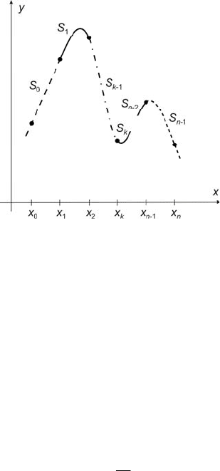
Fig. 4.10 shows the natural spline. Implementing the condition (4.64) in effect
makes the cubic function outside the end-points pass into a straight line.
Fig. 4.10 Natural spline
For the parabolic runout spline, for which
10
MM =
(4.66)
1−
=
nn
MM
(4.67)
Eq. (4.63) can be simplified to the following form
⎥
⎥
⎥
⎥
⎥
⎥
⎥
⎥
⎥
⎦
⎤
⎢
⎢
⎢
⎢
⎢
⎢
⎢
⎢
⎢
⎣
⎡
+−
+−
+−
+−
+−
Δ
=
⎥
⎥
⎥
⎥
⎥
⎥
⎥
⎥
⎥
⎦
⎤
⎢
⎢
⎢
⎢
⎢
⎢
⎢
⎢
⎢
⎣
⎡
⋅
⎥
⎥
⎥
⎥
⎥
⎥
⎥
⎥
⎥
⎦
⎤
⎢
⎢
⎢
⎢
⎢
⎢
⎢
⎢
⎢
⎣
⎡
−−
−−−
−
−
−
)()(2)(
)()(2)(
.
.
)()(2)(
)()(2)(
)()(2)(
6
.
5100..0000
1410..0000
0141..0000
..........
0000..1410
0000..0141
000
0..0015
12
123
432
321
210
2
1
2
3
3
2
1
nnn
nnn
n
n
n
xfxfxf
xfxfxf
xfxfxf
xfxfxf
xfxfxf
M
M
M
M
M
M
(4.68)
Fig. 4.11 presents the parabolic runout spline. Implementing the condition (4.67)
and (4.68) in effect makes the cubic function outside the end-points pass into
a parabola.
For the cubic runout spline, we have
210
2 MMM −=
(4.69)
21
2
−−
−=
nnn
MMM
(4.70)

100 4 Model Development
Fig. 4.11 Parabolic runout spline
and now Eq. (4.63) takes the form
⎥
⎥
⎥
⎥
⎥
⎥
⎥
⎥
⎥
⎦
⎤
⎢
⎢
⎢
⎢
⎢
⎢
⎢
⎢
⎢
⎣
⎡
+−
+−
+−
+−
+−
Δ
=
⎥
⎥
⎥
⎥
⎥
⎥
⎥
⎥
⎥
⎦
⎤
⎢
⎢
⎢
⎢
⎢
⎢
⎢
⎢
⎢
⎣
⎡
⋅
⎥
⎥
⎥
⎥
⎥
⎥
⎥
⎥
⎥
⎦
⎤
⎢
⎢
⎢
⎢
⎢
⎢
⎢
⎢
⎢
⎣
⎡
−−
−−−
−
−
−
)()(2)(
)()(2)(
.
.
)()(2)(
)()(2)(
)()(2)(
6
.
6000..0000
1410..0000
0141..0000
..........
0000..1410
0000..0141
000
0..0006
12
123
432
321
210
2
1
2
3
3
2
1
nnn
nnn
n
n
n
xfxfxf
xfxfxf
xfxfxf
xfxfxf
xfxfxf
M
M
M
M
M
M
(4.71)
Fig. 4.12 presents the cubic runout spline, for which the cubic function outside of
the end-points does not pass into any other function
Fig. 4.12 Cubic runout spline
