Koster A., Munoz X. Graphs and Algorithms in Communication Networks
Подождите немного. Документ загружается.

14 Data Gathering in Wireless Networks 375
For the distributed model, for WGP minimizing flow times in the general inter-
ference model, the performance of algorithm DG is studied by Bonifaci et al. [14].
Again, the performance of the algorithm was studied in a resource augmentation
setting with an increase in speed of factor
σ
, similarly to the centralized model.
We refer to this version as
σ
-speed DG, although the algorithm is identical to DIS-
TRIBUTED GREEDY. Also, they focused on minimizing average flow times instead
of minimizing maximum flow times. The motivation for this objective over the ob-
jective minimizing maximum flow times is based on the proof of the lower bound
of Theorem 14.5. As described above the proof indicates that for a general class of
distributed algorithms, i.e., algorithms which base decisions on random selection,
it is rather unlikely that there exists a constant competitive algorithm for this prob-
lem, even if one allows resource augmentation using extra speed. The same authors
presented the following positive result.
Theorem 14.11. Let 0 <
ε
≤ 1 and
σ
= 6
μ
−1
·log
Δ
·ln(
δ
/
ε
). Then
σ
-speed DG
is in expectation (1+ 3
ε
)-competitive when minimizing the average flow time.
14.5 Conclusion
The chapter surveys recent complexity results and approximation algorithms for
several variants of the wireless gathering problem. It considers different interference
models, the uniform and non-uniform data models, different optimization parame-
ters, and the off-line and online settings of the problem.
Many interesting directions of future work arise from the considered problems.
These include the attempt to close the existing gaps between the upper and lower
bounds for the specific problems. Where good solutions on general graphs are not
possible or not available, the focus on graph classes that are of interest from a prac-
tical point of view is of high importance. In the non-uniform data model many im-
portant questions are still to be resolved. Also, more work remains to be done on
unidirectional antennas with or without buffering capabilities at the nodes. Finally,
especially from a practical perspective, the study of distributed algorithms needs to
be further intensified.
Acknowledgements This work was supported by EU COST action 293 – Graphs and Algorithms
in Communication Networks (GRAAL). Research of the authors was partially supported by the Fu-
ture and Emerging Technologies Unit of EC (IST priority – 6th FP) under contract no. FP6-021235-
2 (project ARRIVAL), by the Dutch BSIK-BRICKS project, by EU ICT-FET 215270 FRONTS,
by MIUR-FIRB Italy-Israel project RBIN047MH9, by ANR-project ALADDIN (France), by the
project CEPAGE of INRIA (France), and by European project COST Action 295 Dynamic Com-
munication Networks (DYNAMO).
376 V. Bonifaci et al.
References
1. Akyildiz, I. F., Su, W., Sankarasubramaniam, Y., Cayirci, E.: Wireless sensor networks: a
survey. Computer Networks 38(4), 393–422 (2002)
2. Ausiello, G., Protasi, M., Marchetti-Spaccamela, A., Gambosi, G., Crescenzi, P., Kann, V.:
Complexity and Approximation: Combinatorial Optimization Problems and Their Approx-
imability Properties. Springer (1999)
3. Bar-Yehuda, R., Goldreich, O., Itai, A.: On the time-complexity of broadcast in multi-hop ra-
dio networks: an exponential gap between determinism and randomization. Journal of Com-
puter and System Sciences 45(1), 104–126 (1992)
4. Bar-Yehuda, R., Israeli, A., Itai, A.: Multiple communication in multihop radio networks.
SIAM Journal on Computing 22(4), 875–887 (1993)
5. Bermond, J. C., Corr
ˆ
ea, R. C., Yu, M. L.: Gathering algorithms on paths under interference
constraints. In: Proceedings of the 6th Italian Conference Algorithms and Complexity, Lecture
Notes in Computer Science, vol. 3998, pp. 115–126. Springer (2006). Full version to appear
in Discrete Mathematics
6. Bermond, J. C., Galtier, J., Klasing, R., Morales, N., P
´
erennes, S.: Gathering in specific
radio networks. In: 8
`
emes Rencontres Francophones sur les Aspects Algorithmiques des
T
´
el
´
ecommunications, pp. 85–88. Tr
´
egastel, France (2006)
7. Bermond, J. C., Galtier, J., Klasing, R., Morales, N., P
´
erennes, S.: Hardness and approxima-
tion of gathering in static radio networks. Parallel Processing Letters 16(2), 165–183 (2006)
8. Bermond, J. C., Galtier, J., Klasing, R., Morales, N., P
´
erennes, S.: Hardness and approxima-
tion of gathering in static radio networks. In: Proc. Foundation and Algorithms for Wireless
Networking, pp. 75–79. Pisa, Italy (2006)
9. Bermond, J. C., Gargano, L., Rescigno, A.: Gathering with minimum delay in tree sensor
networks. In: Proceedings of the 15th International Colloquium on Structural Information and
Communication Complexity, Lecture Notes in Computer Science, vol. 5058, pp. 262–276.
Springer (2008)
10. Bermond, J. C., Peters, J.: Efficient gathering in radio grids with interference. In: Septi
´
emes
Rencontres Francophones sur les Aspects Algorithmiques des T
´
el
´
ecommunications, pp. 103–
106. Presqu’
ˆ
ıle de Giens, France (2005)
11. Bermond, J. C., Yu, M. L.: Optimal gathering algorithms in multi-hop radio tree networks
with interferences. In: Proc. of the Int. Conf. on Ad-Hoc, Mobile, and Wireless Networks, pp.
204–217 (2008)
12. Bertin, P., Bresse, J. F., Sage, B.: Acc
`
es haut d
´
ebit en zone rurale: une solution “ad hoc”.
France Telecom R & D 22, 16–18 (2005)
13. Bonifaci, V., Korteweg, P., Marchetti-Spaccamela, A., Stougie, L.: An approximation algo-
rithm for the wireless gathering problem. Operations Research Letters 36(5), 605–608 (2008)
14. Bonifaci, V., Korteweg, P., Marchetti-Spaccamela, A., Stougie, L.: The distributed wireless
gathering problem. In: Proc. Int. Conf. on Algorithmic Aspects in Information and Manage-
ment, Lecture Notes in Computer Science, vol. 5034, pp. 72–83. Springer (2008)
15. Bonifaci, V., Korteweg, P., Marchetti-Spaccamela, A., Stougie, L.: Minimizing average flow
time in sensor data gathering. In: Proc. 4th Workshop on Algorithmic Aspects of Wireless
Sensor Networks, Lecture Notes in Computer Science, vol. 5389, pp. 18–29. Springer (2008)
16. Bonifaci, V., Korteweg, P., Marchetti-Spaccamela, A., Stougie, L.: Minimizing flow time in
the wireless gathering problem. In: Proceedings of the 25th International Symposium on
Theoretical Aspects of Computer Science, pp. 109–120 (2008)
17. Borodin, A., El-Yaniv, R.: Online computation and competitive analysis. Cambridge Univer-
sity Press (1998)
18. Boukerche, A. (ed.): Handbook of Algorithms for Wireless Networking and Mobile Comput-
ing. Chapman & Hall (2005)
19. Cidon, I., Kutten, S., Mansour, Y., Peleg, D.: Greedy packet scheduling. SIAM Journal on
Computing 24(1), 148–157 (1995)
14 Data Gathering in Wireless Networks 377
20. Coleri, S.: PEDAMACS: Power Efficient and Delay Aware Medium Access Protocol for Sen-
sor Networks. Master’s thesis, University of California, Berkeley (2002)
21. Duckworth, W., Manlove, D., Zito, M.: On the approximability of the maximum induced
matching problem. Journal of Discrete Algorithms 3(1), 79–91 (2005)
22. Florens, C., Franceschetti, M., McEliece, R. J.: Lower bounds on data collection time in sen-
sory networks. IEEE Journal on Selected Areas in Communications 22, 1110– 1120 (2004)
23. Garey, M. R., Johnson, D. S.: Computers and Intractability: A Guide to the Theory of NP-
Completeness. Freeman (1979)
24. Gargano, L.: Time optimal gathering in sensor networks. In: Proceedings of the 14th Interna-
tional Colloquium on Structural Information and Communication Complexity, Lecture Notes
in Computer Science, vol. 4474, pp. 7–10. Springer (2007)
25. Gargano, L., Rescigno, A. A.: Optimally fast data gathering in sensor networks. In: Pro-
ceedings of the 31st Symposium on Mathematical Foundations of Computer Science, Lecture
Notes in Computer Science, vol. 4162, pp. 399–411. Springer (2006)
26. Hromkovi
ˇ
c, J.: Algorithmics for Hard Problems — Introduction to Combinatorial Optimiza-
tion, Randomization, Approximation, and Heuristics. Springer (2001)
27. Klasing, R., Morales, N., P
´
erennes, S.: On the complexity of bandwidth allocation in radio
networks. Theoretical Computer Science 406, 225–239 (2008)
28. Korteweg, P.: Online Gathering Algorithms for Wireless Networks. Ph.D. thesis, Eindhoven
Technical University (2008)
29. Kumar, V. S. A., Marathe, M. V., Parthasarathy, S., Srinivasan, A.: End-to-end packet-
scheduling in wireless ad-hoc networks. In: J. I. Munro (ed.) Proceedings of the 15th Sympo-
sium on Discrete Algorithms, pp. 1021–1030 (2004)
30. Morales, N.: Algorithmique de r
´
eseaux de communication radio modelis
´
es par de graphes.
PhD thesis, Universit
´
e de Nice-Sophia Antipolis (2007)
31. Papadimitriou, C. H.: Computational Complexity. Addison-Wesley (1994)
32. Perkins, C. E. (ed.): Ad Hoc Networking. Addison-Wesley Professional (2001)
33. Pottie, G. J., Kaiser, W. J.: Wireless integrated network sensors. Communications of the ACM
43(5), 51–58 (2000)
34. Raghavendra, C. S., Sivalingam, K. M., Znati, T. (eds.): Wireless Sensor Networks. Springer
(2004)
35. Revah, Y., Segal, M.: Improved algorithms for data-gathering time in sensor networks II: Ring,
tree and grid topologies. In: Proc. of the 3rd IEEE Int. Conf. on Networking and Services
(2007)
36. Revah, Y., Segal, M.: Improved lower bounds for data-gathering time in sensor networks. In:
Proc. of the 3rd IEEE Int. Conf. on Networking and Services (2007)
37. Schmid, S., Wattenhofer, R.: Algorithmic models for sensor networks. In: Proceedings of the
20th International Parallel and Distributed Processing Symposium (2006)
38. Segal, M., Yedidsion, L.: On real time data-gathering in sensor networks. In: Proc. of the 3rd
IEEE Int. Conf. on Mobile, Adhoc and Sensor Systems (2007)
39. Vazirani, V. V.: Approximation Algorithms. Springer, Berlin (2001)
40. Yao, A. C. C.: Probabilistic computations: Towards a unified measure of complexity. In: Proc.
of the 18th Symp. on the Foundations of Computer Science, pp. 222–227 (1977)

Chapter 15
Tournament Methods for WLAN: Analysis and
Efficiency
J
´
er
ˆ
ome Galtier
Abstract In the context of radio distributed networks, we present a generalized ap-
proach for Medium Access Control (MAC) with a fixed congestion window. Our
protocol is quite simple to analyze and can be used in a lot of different situations.
We give mathematical evidence showing that our performance is asymptotically
tight. We also place ourselves in the WiFi and WiMAX frameworks, and discuss
experimental results showing collision reduction of 14% to 21% compared to the
best-known methods. We discuss channel capacity improvement and fairness con-
siderations.
Key words: WLAN, MAC protocol, tournament, CSMA, WiFi, WiMAX
15.1 Introduction and Related Works
Radio networks have received in the past few years a growing interest for their abil-
ity to offer relatively wide band radio networking. Applications cover a large area
of domains, including computer network wireless infrastructures and high speed
Internet access for rural areas.
For instance, in WiFi and WiMAX norms, the underlying mechanism [1, 2] (see
also [19]) is a 2-layer protocol whose first part relies on a derivative of the Binary
Exponential Backoff protocol (BEB). The principle is that when a failure occurs, the
transmission protocol delays the following retransmission by some penalty factor.
The protocol uses a contention window (CW ) mechanism to realize this backoff
mechanism. Roughly speaking, the probability of trying an access to the channel
is 1/CW . When a transmission fails, the station increases CW in order to be less
demanding for future accesses.
J
´
er
ˆ
ome Galtier
Orange Labs, 905 Avenue Albert Einstein, 06921 Sophia Antipolis Cedex, France, e-mail:
jerome.galtier@orange-ftgroup.com
A.M.C.A. Koster, X. Mu
˜
noz (eds.), Graphs and Algorithms in Communication 379
Networks, Texts in Theoretical Computer Science. An EATCS Series,
DOI 10.1007/978-3-642-02250-0
15,
c
Springer-Verlag Berlin Heidelberg 2010

380 J. Galtier
DIFS CRP
...
Failed transmissionSuccessful transmission
DIFS CRP SIFS ACK DIFS CRP SIFS ACKPacket Packet Packet
Successful transmission
Fig. 15.1 A view of the general frame structure
Already much research work has been done to model the CW increase or de-
crease process. Strong simplifying assumptions are at the basis of some models [8],
while other researchers focus on an individual station while considering that the
effect of the several contending terminals on the channel can be represented by an
occupancy probability p
occ
(see [5, 22, 23]), following an earlier popular approach
on CSMA [4, 18].
In fact, those studies show that on average, the contention window mechanism
draws the stations to access the channel with some probability that converges to a
value noted p
acc
(n) which depends on the number of stations simultaneously will-
ing to access the channel. Therefore, several studies have shown that the optimal
behavior is when p
acc
(n)=O(1/n), and proposed some alternative mechanisms to
increase and decrease the contention window in order to reach this value. In [6, 7],
the authors aim at guessing the total number of stations trying to emit in order to
directly set the value CW . In [12], an optimization of the increase or decrease pa-
rameters is done to converge to the optimal channel efficiency in terms of capacity.
In [13] the authors use the observation of idle slots to deduce the probable number
of competing stations. In [14], however, strong evidence is given that, with a dy-
namic number of stations, all the aforementioned studies should be questioned as
the guess for the number of contending stations becomes less and less accurate.
A different branch of CSMA protocols has been initiated by the Hiperlan protocol
[20], a twin standard of 802.11a developed in the same period. In this protocol, the
contention phase is bounded. The contention phase begins for each terminal with the
emission of a burst whose length follows a truncated geometric distribution, and the
terminal having the longest burst wins the right to transmit. If several terminals have
the same longest burst, this results in a collision. A very similar protocol developed
in the context of sensor networks has been called Sift [16].
Another related protocol is the Contention Tree Algorithm [9, 10, 17], or CTA
for short, also called Stack Algorithm [11, 21], which uses a tree to solve contention
problems. Although we also use a tree, our protocol is completely different. This al-
gorithm is basically based on feedback, that is, evidence that a collision occured. In
the radio context, a feedback is costly since it requires an acknowledgement packet.
Instead, we rely on evidence of occupation, that is, the fact that a silent terminal can
detect that one or more terminals are signaling their presence.
In Figure 15.1 we explain how our protocol, the selective tournaments, works. As
in the standard 802.11 approach, the transmission begins with a period of sensing
after the last emission (either a packet or an ACK). After observing a sufficiently
long period with no emission (the DIFS period), the system operates a contention
resolution protocol (CRP) that is supposed to select one station, and only one. Then
the packet is transmitted. If it is correctly received, the receiving station emits an
15 Tournament Methods for WLAN 381
ACK after an SIFS period. This is the end of a transmission period and a new trans-
mission period can begin. If no ACK is received back, the new transmission period
begins immediately after the failed packet, and the stations start the CRP mechanism
just after the DIFS period (note that SIFS < DIFS).
How does the CRP work? In our protocol the time is subdivided into time slots
that correspond to rounds of selection. At the beginning, each terminal emits a signal
on the first time slot with a certain probability. In the case where the station does
not emit, it listens to other signals, and, in the case where it hears at least one other
signal, it retires itself from the selection. This process, called round, is repeated an
appropriate number of times, in order to leave only one remaining station at the end
with the highest probability. This method is used in [3].
15.2 Description of the Tournament Method
The present article generalizes this last method, and presents a mathematical frame-
work to analyze its strenghts and weaknesses. As a result, the improved method
presents a reduction of collision between 13.9% and 21.1%, resulting in a system-
atic gain with respect to the original throughput. The gain to the original 802.11b
norm is as high as 34.1%, achieving the best-known throughput for this family of
protocols. More than that, the new protocol keeps excellent fairness characteristics,
as the Jain index indicates.
More than that, we do not use a fixed number of rounds in the tournament as is
done in CONTI (in [3] a fixed number of six rounds is assumed). We use a variable
number of slots of selection, depending on what was previously heard on the chan-
nel. We tune our experiments to the case where the amount of contending stations
is often between 10 and 100, but our analysis can be very easily extended to any
number of contending stations. By adding a sufficient number of minislots, we can
reduce the number of collisions to an arbitrarily low level. Since adding a minislot
can be statistically more penalizing from the throughput point of view than retrans-
mitting a packet in the case of a collision, a clever balance should be computed to
obtain an optimal throughput. In the following, an entry of our protocol will be the
variable E
f
(r(1),...,r(k)), which states whether the collision resolution protocol
should be stopped at round k or not.
The key for obtaining good results is in the choice of the probabilities with which
a station will decide to keep silent or emit a signal in the CRP phase. Each station
takes into account whether signals were emitted or not in the previous rounds to
adapt its probability of emission.
In the following, we call try-bit and denote by r(t) the information that at least
one station has emitted a signal on the tth round.
In Figure 15.2, we show how the choice of p – the probability that a station emits
at a given round of selection – evolves in the course of the rounds of selection and
in the function of the previous try-bits chosen by the terminal. The first value (in
Figure 15.2, p = 0.02) is unique for all the terminals. During the second round, if
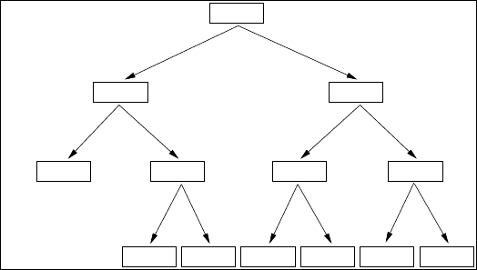
382 J. Galtier
the terminal has emitted a signal in the first round (which we denote r(1)=1), the
protocol chooses the left part of the tree, and uses p
1
= 0.33 for the second round. If
on the other hand the terminal did not emit, and did not hear any signal from other
terminals (r(1)=0), then the protocol chooses the right part of the tree and uses
p
0
= 0.12 for the second round. In the case where the terminal did not emit and
actually hears a signal from another station, it retires and leaves to other stations the
right to send the following packet. As a result, the probability in the second round
is necessarily p
r(1)
. The realization of the second round will determine the value of
r(2), and the third round will be governed by the probability p
r(1)r(2)
in the tree of
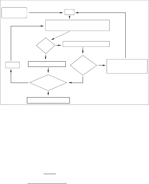
Figure 15.2. We plot the whole process in Figure 15.3. Note that each station has a
local try-bit R(t) at round t which equals r(t) as long as the station is not eliminated.
In Figure 15.3, we also make use of the pf and Ef functions. pf is a function
that, given the values R(1)...R(t −1) of the previous rounds of the tournament,
outputs a probability P[R(t)] of emission of a signal during the actual round. In the
following, we will note w = “R(1)
...“R(t)
as the word containing the history of
the tournament and use the notation p
w
to model what will be pf[R(1),...,R(t −1)].
Also Efis a function of R(1)...R(t) which indicates to the terminal that in the case
of success for round t, it has to proceed to emit the packet (Ef= yes) or start another
round of selection (Ef = no). Note also that in the bottom-left part of Figure 15.2,
only three rounds of elimination are performed, while four are requested in the other
parts of the tree. Depending on the previous states, that is, on r(1),r(2),...,r(t),
our protocol can decide to perform the transmission. In the case of Figure15.2, until
the third round, three successive signals have been emitted, so the system forsees
that one station is attempting to communicate with high priority, and proceeds to
transmission.
We manage to find a tight approximation of the behavior of this protocol when
the number of rounds increases. More precisely, if we denote by q
n
the probability
that n stations try to emit in the system, and if we introduce the function
fourth round
p=0.02
r(2)
r(3)
10 1
1100
0
r(1) 1 0
p11=0.45 p10=0.39 p01=0.32 p00=0.25
p1=0.33 p0=0.12
p101=0.45 p100=0.44 p011=0.43 p010=0.43 p010=0.42 p010=0.42
01
}
}
}
round
first
round
third
second
round
Fig. 15.2 Choice of the values of p in the course of the rounds of selection
15 Tournament Methods for WLAN 383
Emission of a signal
?
yes
no
Is there
no
signal?
another
yes
(signal(s) + packet(s))
of the emissions
Waiting of the end
a new packet
Emission of
Emission of the packet
t:=1
Drawing of the value R(t) in {0,1}
Listening to other signals
t:=t+1
R(t)=0
with P[R(t)=0]=pf(R(1),...,R(t−1))
no
yes
Ef(R(1),...,R(t))?
Fig. 15.3 Global diagram for the rounds of selection in a terminal
f (x)=
∑
n≥1
q
n
x
n
, (15.1)
then we can show that, tuning the p coefficients to this probability space, the rate of
collision 1 −
ρ
observed if the protocols stops after k rounds will be fairly approxi-
mated by
1−
ρ
≈
.
1
0
1
f
(t)dt
2
2
k+1
.
The article is organized as follows. A mathematical modeling in the next section
investigates analytically the optimization issues raised by the problem of the choice
of the p’s, and gives some tight bounds for this question. The reader that desires
to know the protocol without the mathematics can skip this section. A practical
implementation of the mathematical ideas, allowing the computation of the values
of the p’s, is given in Section 15.3, which gives a new protocol for the WiFi/WiMAX
networks. Here again, the reader will not need to program the whole framework to
implement and reproduce our protocol, which is described in terms of parameters in
Table 15.2. Finally, our protocol is compared with other ones in Section 15.4, where
some numerical results are presented. A summary of the notations used throughout
the chapter is given in Table 15.1.
15.3 Mathematical Analysis
During the mathematical part of the analysis, we study the case where the CRP stops
after k rounds. In the following we denote by m the number 2
k
.

384 J. Galtier
Table 15.1 Notations used in this chapter
k Number of rounds of selection. z
i
Riemann steps for f
in [0,1], i ∈{0,...,m}.
m 2
k
.
ϕ
Continuous function in [0,1] to be approxi
r(t) Try-bit at the tth round of selection, -mated.
t ∈{1,...,k}.
ψ
Piecewise constant function that approximate
R(t) Local try-bit (at a station) at the tth
ϕ
.
round of selection, t ∈{1,...,k}. c
m
Best approximation gap for the approximation
q
n
Probability that n station try to emit. of
ϕ
with m pieces.
w Word in the alphabet {0,1}.
σ
Increasing function from IN to IN that
l(w) Length of the word w. emphasizes extraction.
#(w) Binary value represented by wAFunction of IR
m+1
to IR that reaches approxi-
p Probability that a station emits a sig- mation for
ϕ
.
nal at the first round of selection.
¯
h Density step function defined after z
·
, see equa
p
w
Probability that a non-eliminated sta- tion (15.6).
tion emits a signal at the round h
∗
Density function that minimizes
l(w)+1, given that the preceding
.
1
0
f
(t)/h(t)dt, see Proposition 15.2.
try-bits where r(1),...,r(l(w)) = w.
ˆ
h Density function taken for the algorithmic
f Generating function of q
.
, see equation choices of z
·
,
ˆ
h(x)=
1
f
(x).
(15.1). M Large number compared to m.
f
w
Generating function of the number of L Level variable (L = 2
k−l(w)−1
).
non-eliminated stations, in the event w. N Maximum number of foreseen stations.
g Generating function of the number of
α
Parameter to set the values of q
·
, see equa-
non-eliminated stations after k rounds. tion (15.13).
ρ
Success rate (as opposed to the colli- x
i
In the experiments, amount of packets that an
sion rate). individual station has emitted.
δ
w
Local step, see equation (15.2).
π
w
In the experiments, the probability that the se-
y
w
Cumulative step, see equation (15.3). quence w will be used for signaling.
We denote by q
n
the probability that n stations try to emit in the system. We have
necessarily q
n
≥0 and
∑
n≥1
q
n
= 1. We introduce f , which in the following we will
call the generating function of the distribution of stations, defined by:
f (x)=
∑
n≥1
q
n
x
n
.
We try now to characterize the distribution after the transmission on the first
mini-slot. Let f
1
and f
0
be generating functions for the number of stations still in
contention depending, respectively, on whether or not there was a transmission in the
previous slot. If every station emits a signal with probability p, then the probability
that n stations emit is given by
P[n stations emit a signal]=
∑
i≥n
(
i
n
)q
i
p
n
(1−p)
i−n
.
Therefore, the distribution of the number of stations that emit is characterized by a
function f
1
analog of f , defined by
f
1
(x)=
∑
i≥1
P[i stations emit a signal]x
i
,
and we deduce logically that
15 Tournament Methods for WLAN 385
f
1
(x)=
∑
n≥1
∑
1≤i≤n
(
n
i
)q
n
p
i
(1−p)
n−i
x
i
=
∑
n≥1
q
n
[(px + 1 − p)
n
−(1−p)
n
]
= f(px + 1 − p) − f (1 − p).
Similarly, in the event where no signal has been emitted in the first round, we can
deduce some information on the distribution of the number of stations. Indeed, the
probability that n stations remain silent is (1 −p)
n
. Therefore, if we write
f
0
(x)=
∑
i≥0
P[i stations are present and remain silent]x
i
then we obtain
f
0
(x)=
∑
i≥0
q
i
x
i
(1−p)
i
= f ((1 − p)x).
And we see that at the end of the first round of selection, the distribution of the
whole set of surviving station can be known by the mathematical function f
0
+ f
1
.
We can also note that the distribution in the case where the event r(0) occurs (either
0or1)isgivenby f
r(0)
/ f
r(0)
(1).
By extension, if we let w be a word in the alphabet {0, 1}, and w0(orw1) the
same word to which the letter “0” (or “1”) is added, and if we let p
w
and f
w
,re-
spectively, be the probability and generating function corresponding to step w, then
(setting f
/0
= f ) the following inductive formulas hold:
f
w1
(x)=f
w
(p
w
x + 1 − p
w
) − f
w
(1−p
w
)
f
w0
(x)=f
w
((1−p
w
)x)
We observe that the probability of the event of the choice w = r(1)...r(t) is
f
w
(1). Given that the event w occurs, the distribution of the number of stations is
characterized by f
r(1)...r(k)
/ f
r(1)...r(k)
(1). If we denote by l(w) the length of the word
w, then the global distribution g for all the event space after k rounds of selection is
given by the sum of all the f
w
’s that correspond to an event after k rounds (this is
true if and only if l(w)=k, since E
f
(w) is true when l(w) reaches k), and therefore,
g(x)=
∑
w:l(w)=k
f
w
(x).
The probability of success
ρ
of the rounds of selection is the probability that only
one station remains. It is given by the first term of the integral series of g, that is,
g
(0). Therefore,
ρ
=
∑
w:l(w)=k
f
w
(0).
In the following we evaluate the value of f
w
(0). We therefore denote, for any word
w in the alphabet {0,1}, the quantity defined inductively by
δ
/0
= 1 and
δ
w0
=(1−p
w
)
δ
w
δ
w1
= p
w
δ
w
(15.2)