Koster A., Munoz X. Graphs and Algorithms in Communication Networks
Подождите немного. Документ загружается.

14 Data Gathering in Wireless Networks 365
Theorem 14.4. Unless P = NP, no polynomial-time algorithm can have approxima-
tion ratio better than
Ω
(m
1/3
) for FMAX-WGP in the general interference model,
even when d
T
= d
I
= 1.
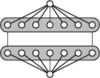
Proof. Let (G, k) be an instance of IBM, G =(U,V,E). We construct a four-layer
network with a unique source o (first layer), a clique on U and a clique on V (middle
layers), and a sink s (last layer). Source o is adjacent to each node in U, and s to
each node in V. The edges between U and V are the same as in G (see Figure 14.4).
We set d
T
= d
I
= 1.
o
s
G
U
V
Fig. 14.4 The construction in the proof of Theorem 14.4
The FMAX-WGP instance consists of m =(1 −1/
α
)
−1
(1 + k/
α
)(2k + 1)k =
Θ
(k
3
) packets with origin o. They are divided into m/k groups of size k. Each packet
in the hth group has release date (k + 1)h, h = 0, ..., m/k −1. Rounds (k + 1)h to
(k + 1)(h + 1) −1 together are a phase.
We prove that if G has an induced matching of size k, there is a gathering schedule
of cost 2k + 1, while if G has no induced matching of size more than k/
α
,every
schedule has cost at least (2k + 1)k =(2k + 1)
Θ
(m
1/3
). The theorem then follows
directly.
Assume G has an induced matching M of size k,say(u
i
,v
i
), i = 0...k −1. Then
consider the following gathering schedule. In each phase, the k new packets at o are
transmitted, necessarily one by one, to layer U while old packets at layer V (if any)
are absorbed at the sink; then, in a single round, the k new packets move from U
to V via the matching edges. More precisely, each phase can be scheduled in k + 1
rounds as follows:
1. for i = 0, ..., k −1 execute in round i the two calls (o,u
i
) and (v
i+1modk
,s);
2. in round k, execute simultaneously all the calls (u
i
,v
i
), i = 0, ..., k −1.
The maximum flow time of the schedule is 2k + 1, as a packet released in phase h
reaches the sink before the end of phase h + 1.
In the other direction, assume that each induced matching of G is of size at most
k/
α
. By Proposition 14.2, at most k/
α
calls can be scheduled in any round from
layer U to layer V. We ignore potential interference between calls from o to U and
calls from V to s; doing so may decrease the cost of a schedule. As a consequence,
we can assume that each packet follows a shortest path from o to s. Notice however
that, due to the cliques on the layers U and V , no call from U to V is compatible
with a call from o to U, or with a call from V to s.
366 V. Bonifaci et al.
Let m
o
and m
U
be the number of packets at o and U, respectively, at the beginning
of a given phase. Also, let
β
= 1 + k/
α
. We associate with the phase a potential
value
ψ
=
β
m
o
+ m
U
, and we show that at the end of the phase the potential will
have increased proportionally to k.Letc
o
and c
U
denote the number of calls from o
to U and from U to V , respectively, during the phase. Since a phase consists of k + 1
rounds, and in each round at most k/
α
calls are scheduled from U to V,wehave
c
o
+ c
U
/(k/
α
) ≤ k + 1, or, equivalently since k/
α
=
β
−1,
(
β
−1)c
o
+ c
U
≤ (
β
−1)(k + 1). (14.1)
If m
o
, m
U
are the number of packets at o and U at the beginning of the next phase,
and
ψ
=
β
m
o
+ m
U
is the new potential, we have
m
o
= m
o
+ k −c
o
m
U
= m
U
+ c
o
−c
U
ψ
−
ψ
=
β
(m
o
−m
o
)+m
U
−m
U
=
β
(k −c
o
)+c
o
−c
U
=
β
k −(
β
−1)c
o
−c
U
≥
β
k −(
β
−1)(k + 1)
= k −(
β
−1)
=(1−1/
α
)k
where the inequality uses (14.1).
Thus, consider the situation after m/k phases. The potential has become at least
Ψ
=(1 −1/
α
)m. By definition of the potential, this implies that at least
Ψ
/
β
=
(1 −1/
α
)(1 + k/
α
)
−1
m =(2k + 1)k packets reside at either o or U; in particular,
they have been released but not yet absorbed at the sink. Since the sink cannot
receive more than one packet per round, this clearly implies a maximum flow time
of (2k + 1)k =(2k + 1)
Θ
(m
1/3
) for one of these packets. #$
A similar construction shows that the same problem with minimization of total
flow time F
SUM-WGP cannot be approximated within a ratio better than
Ω
(m
1−
ε
)
for any 0 <
ε
< 1 [15]. We also notice that a similar instance as that used in Sec-
tion 14.3.1 constructed for proving inapproximability of shortest paths following
algorithms for C
MAX-WGP can be constructed here to prove that shortest paths
following algorithms cannot approximate optimal solutions of F
MAX-WGP and
F
SUM-WGP within a ratio better than
Ω
(m).
For the distributed model, Bonifaci et al. [14] provided lower bounds for F
MAX-
WGP which do not depend on the assumption P = NP. They consider a scenario in
which the network is partitioned into layers based on distance to the sink. They as-
sume that interference conflicts between transmissions from one layer of the tree to
the next are resolved randomly: whenever several transmissions from a layer occur
in the same round, only a uniformly chosen one succeeds; this is called the random
selection model. This assumption seems natural for distributed algorithms, as they
have no simple means of coordinating the transmitting nodes (or more precisely,
14 Data Gathering in Wireless Networks 367
coordinating the transmitting nodes is as hard as the original communication task).
For distributed algorithms following a random selection model they present the fol-
lowing lower bound.
Theorem 14.5. In the random selection model the approximation ratio of any algo-
rithm for F
MAX-WGP is at least
Ω
(logm).
In fact, Bonifaci et al. [14] argue that even resource augmentation using speed as a
resource is not likely to improve this lower bound. The reason is that the lower bound
is due to an adversarial selection of which packet to advance; and the probability of
obtaining such a selection depends on the number of packets, and not on the speed
of the algorithm.
14.4 Online Algorithms
14.4.1 Minimizing Makespan
14.4.1.1 Omnidirectional Antennas
Several authors have presented centralized online algorithms for omnidirectional
WGP. The first algorithm, P
IPELINE, was presented by Bermond et al. [7, 8]. The
algorithm was analyzed in an off-line context, but can be implemented in an online
setting. The idea of the algorithm is to pipeline packets towards the sink by parti-
tioning the graph into intervals. The lengths of the intervals are chosen such that
packets can advance in parallel without interfering with each other.
First, we introduce some notation to facilitate the exposition of the algorithm.
An important concept used in this and other algorithms is that of critical radius.
The critical radius R
∗
is the greatest integer R such that no two nodes at distance
at most R from s can receive a packet in the same round. It is not hard to show
that R
∗
≥
/
d
I
−d
T
2
0
(see, for example, [7, 8]). The critical region is the ball centered
at s of radius R
∗
. Thus, at any round at most one node in the critical region can
receive a packet. We define K
∗
=
R
∗
+1
d
T
≥ 1 and K = 1 +
d
I
+1
d
T
. Roughly stated,
K gives an upper bound on the number of rounds during which a packet needs to be
forwarded before a new packet can be safely forwarded from the same origin over
the same path, while K
∗
gives a lower bound on the number of rounds during which
a packet has to move inside the critical region, assuming it starts outside. We also
let K
0
= 1 +
R
∗
d
T
,Rad= max
u∈V
d(u, s), and L = 1 +
Rad−K
0
d
T
Kd
T
.
The algorithm partitions the set of distances to the sink [1,Rad] into L intervals
I
0
, ..., I
L−1
. These are defined by I
0
=[1,K
0
d
T
] and, for i = 1, ..., L −1, I
i
=
[K
0
d
T
+ 1 +(i −1)Kd
T
,K
0
d
T
+ iKd
T
].
Additionally, each I
i
is split into areas of length d
T
,soI
0
is split into K
0
areas
I
j
0
=[K
0
d
T
+ 1 − jd
T
,K
0
d
T
−( j −1)d
T
], j = 1, ..., K
0
; and I
i
, i = 1, ..., L −1is
split into K areas I
j
i
=[K
0
d
T
+ 1 + iKd
T
− jd
T
,K
0
d
T
+ iKd
T
−( j −1)d
T
], j = 1,
368 V. Bonifaci et al.
..., K. We denote the set of vertices whose distance is in I
i
(respectively I
j
i
)byV
i
(respectively V
j
i
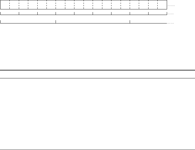
). Figure 14.5 shows a partition with K = 4,K
0
= 3, d
T
= 2.
$I_2$
1 2 3 4 6 7 9 11 12 13 14 15 16 17851810
$I_0^3$ $I_0^2$ $I_0^1$ $I_1^4$ $I_1^3$ $I_1^2$ $I_1^1$ $I_2^4$ $I_2^3$
$I_0$
$I_1$
Fig. 14.5 Partitioning of distance intervals for K = 4,K
0
= 3, d
T
= 2
We are now in position to describe the algorithm (Algorithm 14.1).
Algorithm 14.1 PIPELINE
The algorithm works in phases. Each phase, except possibly the last, consists of K rounds t
j
,
j = 1,...,K. The algorithm uses the concepts of intervals and areas to construct a set of feasible
calls in each round.
for each phase do
for each round t
j
, j = 1,2,...,K do
Select in each interval I
i
avertexu
j
i
in V
j
i
with an available packet to transmit (if such
a vertex exists). Vertex u
j
i
calls the closest vertex in the preceding area, i.e., if d(u
j
i
,s)=
K
0
d
T
+1+iKd
T
− jd
T
+
α
for some 0 ≤
α
< d
T
,thenu
j
i
calls a vertex v such that d(v,s)=
K
0
d
T
+iKd
T
− jd
T
. This means that if i = 0and j < K
0
(or i > 0and j < K)thenv ∈V
j+1
i
,
if i > 0and j = K then v ∈V
1
i−1
,andifi = 0andj = K
0
then v = s.
We claim that PIPELINE creates a feasible schedule for WGP. First, let us show
that for any round the calls scheduled by P
IPELINE are all pairwise compatible. In-
deed, consider two calls (u,v) =(u
,v
) of the same round t
j
. Then d(u,s)=K
0
d
T
+
1+iKd
T
− jd
T
+
α
,forsomei ≥ 0,0 ≤
α
< d
T
, and d(v
,s)=K
0
d
T
+ i
Kd
T
− jd
T
for some i
= i (as v = v
). Therefore, d(u,v
) ≥|(i
−i)Kd
T
−1−
α
|≥d
I
+d
T
−
α
≥
d
I
+1. Similarly one can show d(u
,v) ≥d
I
+1, and the calls are compatible. To see
why the algorithm delivers all the packets, observe that after a phase of K rounds,
the protocol ensures that if a vertex of V
i
contains a packet, then the last vertex of
V
i−1
has received a new packet.
To illustrate P
IPELINE we show one phase of the algorithm in Figure 14.6.
Bonifaci et al. [13] presented a class of online centralized algorithms for C
MAX-
WGP, called P
RIORITY GREEDY.InaPRIORITY GREEDY algorithm each packet
is assigned a unique priority based on some algorithm-specific rules, and the priority
ordering does not change over time. Then, in each round, packets are considered in
order of decreasing priority and are sent towards the sink as far as possible while
avoiding interference with higher priority packets. Thus, the schedule output by the
algorithm is feasible by construction.
14 Data Gathering in Wireless Networks 369
15 16 17851810
I
3
0
I
2
0
I
1
0
I
4
1
I
3
1
I
2
1
I
1
1
I
4
2
I
3
2
I
0
I
1
I
2
1s 2 3 4 6 7 9 11 12 13 14
Fig. 14.6 A phase of PIPELINE, consisting of K = 4 rounds. Here, packets are represented as small
balls. Notice that packets in the same cell are at the same distance from the sink, but they can be in
different vertices
Algorithm 14.2 PRIORITY GREEDY
for each round t = 0,1,2,... do
Consider the available packets in order of decreasing priority, and send each packet as far as
possible along a shortest path from its current node to the sink, without causing interference
with any higher-priority packet.
Both Bermond et al. and Bonifaci et al. use similar concepts to derive upper
bounds on their algorithms, as well as a lower bound on the makespan of an off-line
optimal solution [7, 8, 13].
The lower bound on the completion time of any schedule is based on the obser-
vation that at most one packet can be sent from a node within the critical region. Let
δ
j
=
d(v
j
,s)
d
T
, the minimum number of calls required for packet j to reach s. Define
also
π
j
= min{
δ
j
,K
∗
} and R
j
= r
j
+
δ
j
−
π
j
. Informally,
π
j
gives the number of
rounds during which packet j has to move inside the critical region (irrespective of
whether it originated inside or outside of it); R
j
is the first possible time at which
packet j can reach the border of the critical region. The following bound on the cost
of an optimal solution can be proved by considering only the processing that has to
be done inside the critical region [13].
Lemma 14.1. Let S ⊆ J be a nonempty set of packets, and let C
∗
i
denote the com-
pletion time of packet i in some feasible schedule. Then there is k ∈ S such that
max
i∈S
C
∗
i
≥ R
k
+
∑
i∈S
π
i
.
We sketch the idea behind the upper bound on the completion times; the sketch
is based on the upper bound proof of the P
RIORITY GREEDY algorithm. The idea is
that if a packet is delayed, i.e., it is not sent as far as possible in each round until it
reaches the sink, then this packet must be close to some other packet that is sent in
that round. As a result we can provide a bound on the completion time of a packet
by relating it to the completion time of another packet that delays this packet. This
provides an upper bound on the makespan of a set of packets. Formally, we say that
packet j is blocked in round t if t ≥ r
j
but j is not sent over distance d
T
in round
370 V. Bonifaci et al.
t. Note that in a PRIORITY GREEDY algorithm a packet can only be blocked due to
interference with a higher priority packet. We define the following blocking relation
on a P
RIORITY GREEDY schedule: k ≺ j if in the last round in which j is blocked,
k is the packet closest to j that is sent in that round and has a priority higher than j
(ties broken arbitrarily). The blocking relation induces a directed graph F =(J, A)
on the packet set J with an arc (k, j) for each k, j ∈ J such that k ≺ j. Observe that,
for any P
RIORITY GREEDY schedule, F is a directed forest and the root of each tree
of F is a packet which is never blocked. For each j,letT ( j) ⊆ F be the tree of F
containing j, b( j) ∈ J be the root of T( j), and P( j) be the set of packets along the
path in F from b( j) to j.
Lemma 14.2. For each packet j ∈JinaP
RIORITY GREEDY schedule, C
j
≤R
b( j)
+
(K/K
∗
) ·
∑
i∈P( j)
π
i
.
Bonifaci et al. [13] considered a particular P
RIORITY GREEDY algorithm called
RPG in which packet j has higher priority than packet k if R
j
< R
k
(ties broken
arbitrarily). Combining Lemmas 14.1 and 14.2 they proved the following theorem.
Theorem 14.6. RPG is K/K
∗
-competitive for CMAX-WGP.
Similarly, Bermond et al. [7] presented the following theorem.
Theorem 14.7. P
IPELINE is K/K
∗
-competitive for CMAX-WGP without release
dates.
The exact ratio depends on d
T
and d
I
, but is always bounded: it is straightforward
to verify that 2 ≤K/K
∗
≤4 for all d
T
and d
I
, while K/K
∗
≤3ford
I
= d
T
. Similarly,
Korteweg [28] proved that P
RIORITY GREEDY is (K/K
∗
+ 1)-competitive for any
fixed priority on the packets, using Lemmas 14.1 and 14.2. An interesting open
problem is whether there exists a polynomial-time approximation scheme, or a (1+
ε
)-approximation algorithm for general graphs for small values of
ε
> 0.
Notice that the algorithms P
IPELINE and PRIORITY GREEDY can be imple-
mented using only local information. Namely, it suffices that a node is informed
about the state of nodes within distance d
I
+ 1.
Kumar et al. [29] presented a decentralized algorithm for packet routing under the
distance-2 interference model. The authors presented an O(
Δ
log
2
n)-approximation
algorithm, where
Δ
is the maximum graph degree and n is the number of nodes.
Their algorithm assumes that each node knows upper bounds on the maximum num-
ber of packets per node and the network diameter. The first assumption seems re-
strictive from a practical point of view, where packets arrive online over time. The
algorithm proceeds in phases, and at the start of each phase nodes communicate with
nodes up to a distance 3 to determine interference-free schedules for the round in
the next phase. As such the algorithm, like those discussed above, is decentralized,
but not distributed in the sense that nodes use information about neighboring nodes.
Bar-Yehuda et al. [4] considered a distributed algorithm for C
MAX-WGP in the
special case where d
T
= d
I
= 1 and there are no release dates. We refer to their
algorithm as D
ISTRIBUTED GREEDY (DG). The idea behind DG is the following.

14 Data Gathering in Wireless Networks 371
To reduce interference between nodes, DG partitions nodes into layers, and assigns
a label to nodes in a layer. A layer is a set of all nodes at the same distance from the
sink. A node at distance d from the sink is assigned label d mod 3. Each node can
be either active during a round or inactive; only active nodes will transmit a packet.
A node will not be active if its packet buffer is empty.
DG uses a procedure to establish communication from a set of active nodes. The
procedure, first introduced and studied by Bar-Yehuda, Goldreich, and Itai [3], is
called D
ECAY and requires 2log
Δ
rounds; the time needed for a single execution of
the procedure is called a phase.
Algorithm 14.3 DECAY(u,v)
for j = 1,2,...,2log
Δ
do
u sends to v the oldest packet from its buffer;
u deactivates itself for the rest of the phase with probability 1/2.
In fact, the original description does not describe which packet v to advance from
the buffer, because for the analysis of completion times the choice of this packet is
not relevant. For flow times the choice can be relevant; hence, we choose to advance
the oldest packet. We now present the description of the D
ISTRIBUTED GREEDY
algorithm (Algorithm 14.4).
Algorithm 14.4 DISTRIBUTED GREEDY (DG)
for each phase k = 1,2,... do
Activate each node with label k mod 3 that has a nonempty packet buffer;
Execute D
ECAY(u,parent(u)) in parallel for each active node u.
Although the algorithm does not model acknowledgement of packets explicitly,
it is easy to include them, e.g., by doubling the number of rounds, having com-
munication in odd rounds and acknowledgements in even rounds, as observed by
Bar-Yehuda et al. Using this, we can assume that successful receipt of a packet (by
the parent of the sending node in the communication tree) is acknowledged imme-
diately. Only at that time does it get removed from the sender’s buffer.
By the transmission protocol in DG, where in phase k only nodes of layer k
mod 3 transmit, if two nodes transmit, then either they are at the same layer or they
are at least distance 3 apart. Hence, in DG two nodes can only interfere if both
sender nodes are in the same layer.
A superphase consists of three consecutive phases. Another important ingredient
in the analysis of DG is the following, proved by Bar-Yehuda et al. [4].
Theorem 14.8. Let i be any layer of the tree containing some packet at the beginning
of a superphase. There is probability at least
μ
= e
−1
(1 −e
−1
) that during this
superphase DG sends successfully a packet from at least one node u in layer i to the
parent node of u in the communication tree.
372 V. Bonifaci et al.
This theorem shows that, during a superphase, each nonempty layer forwards
a packet with probability
μ
to the following layer. Notice however that there is
no guarantee on which particular packet is advanced. The use of superphases and
labels, i.e., a synchronous model, is essential to the proof of Theorem 14.8. If the
D
ECAY procedure is applied in an asynchronous model, it is not clear whether a
similar constant probability
μ
is attainable.
Theorem 14.8 suffices to bound the completion time of packets in a schedule
constructed by DG.
Theorem 14.9. D
ISTRIBUTED GREEDY is in expectation O(log
Δ
)-competitive for
C
MAX-WGP without release dates, and d
I
= d
T
= 1.
14.4.1.2 Special Topologies
The hardness results for C
MAX-WGP on general graphs of Section 14.3 motivate
the study of specific topologies, such as the path, balanced stars, and the two-
dimensional grid. With the additional assumption that the data is uniform (every
node holds exactly one packet) it is possible to provide algorithms whose perfor-
mance differs only by an additive constant from the theoretical minimum. We are
not aware of studies for specific topologies in the case of non-uniform data (in par-
ticular, it is unknown whether optimal polynomial-time algorithms are possible for
path or tree topologies), although it is certainly possible to at least improve the ap-
proximation guarantees in this setting.
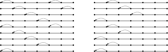
As an example of the uniform data model on a specific topology, Figure 14.7
shows an optimal gathering schedule using 18 rounds for a path of seven vertices
(each having one data packet), with d
T
= 1, d
I
= 2, and s = 0. The schedule has
a regular structure and this regularity can be exploited to give a general algorithm
for paths whose cost differs by the optimal one only by an additive constant term
(though the constant may depend on d
T
and d
I
).
21$s=0$ 3 4 5
6
21$s=0$ 3 4 5
6
21$s=0$ 3 4 5
6
21$s=0$ 3 4 5
6
21$s=0$ 3 4 5
6
21$s=0$ 3 4 5
6
21$s=0$ 3 4 5
6
1
2
3
4
5
6
7
21$s=0$ 3 4 5
6
8
21$s=0$ 3 4 5
6
9
21$s=0$ 3 4 5
6
21$s=0$ 3 4 5
6
21$s=0$ 3 4 5
6
21$s=0$ 3 4 5
6
21$s=0$ 3 4 5
6
21$s=0$ 3 4 5
6
21$s=0$ 3 4 5
6
21$s=0$ 3 4 5
6
17
21$s=0$ 3 4 5
6
10
11
12
13
14
15
16
18
Fig. 14.7 A gathering schedule in the path when d
T
= 1, d
I
= 2, and every vertex has one packet
to send to the sink s = 0
In fact, the uniform model has first been studied in the case of specific graph
topologies for specific values of d
I
and d
T
. In particular, the case d
T
= 1 was studied
in [5] for the case where the graph is a path, and in [10] for the case where the graph
14 Data Gathering in Wireless Networks 373
is the two-dimensional square grid. An optimal algorithm for trees when d
T
= d
I
= 1
is given by Bermond and Yu [11].
Bermond et al. [6, 30] consider the uniform model for paths and grids, for any
value of d
T
. Even though their algorithms do not match the lower bounds, they are
again larger by an additive constant that depends only on d
I
and d
T
. The authors
also study the case of stars and show that the general lower bound of [7, 8] is tight
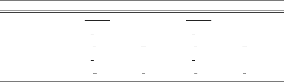
up to a constant that does not depend on the size of the network. Table 14.1 shows
the main results of Bermond et al. [6, 30]. The notation is the following:
• LB (UB) is a lower bound (upper bound) on the number of rounds for gathering
in the corresponding topology.
• P
n
is the path with n vertices 0,1,...,n −1. Vertex i is adjacent to vertex i + 1
for any i = 1, ..., n −2. Therefore, the sink s is simply an integer such that
0 ≤ s ≤n −1.
• S
K,l
is the balanced spider graph with K branches. S
K,l
consists of K copies of P
l
(called branches) sharing a common extreme, the sink s.
• G
2
(p,q) is the two-dimensional grid, i.e., the graph G =(V, E) where V = {(i, j) :
−p ≤ i ≤ p,−q ≤ j ≤ q}.Son =(2p + 1)(2q + 1), and (x, y) and (x
,y
) are
connected when |x −x
|+ |y −y
| = 1. We assume that p,q ≥ d
I
+ d
T
+ 1 and
s =(0, 0).
In Table 14.1, O(1) is used to denote a constant that may depend on d
I
and d
T
but not on the size n of the network.
Table 14.1 Approximation results for gathering in specific topologies
Topology LB UB
P
n
d
I
+d
T
+1
d
T
max[s,n−s] −O(1)
d
I
+d
T
+1
d
T
max[s,n−s]+O(1)
S
K,l
,
d
I
/d
T
odd
1
2
(1+
d
I
/d
T
)n−O(1)
1
2
(1+
d
I
/d
T
)n+ O(1)
S
K,l
,
d
I
/d
T
even
1
2
d
I
/d
T
n +
n
K
−O(1)
1
2
d
I
/d
T
n +
n
K
+ O(1)
G
2
(p,q),
d
I
/d
T
odd
1
2
(1+
d
I
/d
T
)n−O(1)
1
2
(1+
d
I
/d
T
)n+ O(1)
G
2
(p,q),
d
I
/d
T
even
1
2
d
I
/d
T
n +
n
4
−O(1)
1
2
d
I
/d
T
n +
n
4
+ O(1)
14.4.1.3 Unidirectional Antennas
We discuss here some results for gathering problems with unidirectional antennas.
Florens et al. [22] study makespan minimization in a model where each each node
is equipped with directional antennas and has no buffering capacity. Furthermore,
it is assumed that a node cannot receive and send simultaneously, that the com-
munication radius is 1, and that there is no interference but each node can only
receive one message at a time. Under these assumptions, Florens et al. give optimal
(polynomial-time) gathering algorithms for path and tree networks. Their work has

374 V. Bonifaci et al.
been extended to general graphs in the uniform case by Gargano and Rescigno [25].
Other results for specific topologies are discussed by Revah and Segal [35, 36] and
Segal and Yedidsion [38].
A discussion of some algorithmic and graph-theoretic problems related to wire-
less data gathering with minimum makespan is contained in [24]. Finally, another
related model can be found in Klasing et al. [27], where the authors study the case
in which steady-state flow demands between each pair of nodes have to be satisfied.
14.4.2 Minimizing Flow Times
Most literature on gathering problems focuses on minimizing completion times. In
this subsection we highlight some results on minimizing flow times. First, we con-
sider the centralized model. Bonifaci et al. [16] analyzed F
MAX-WGP in the general
interference model. For this version they analyzed the performance of a particular
P
RIORITY GREEDY algorithm. Because it follows from Theorem 14.4 that there is
no constant approximation algorithm for this problem, unless P = NP,theyused
resource augmentation to analyze the quality of the algorithm. They study a variant
of P
RIORITY GREEDY which orders packets based on release dates, i.e., packet j
precedes k if r
j
≤r
k
; ties (r
j
= r
k
) are broken arbitrarily. They call this variant FIFO
after the well known first-in-first-out algorithm in scheduling theory, although in this
case the term FIFO refers to the priority ordering; observe that the first packet in the
system does not have to arrive earliest at the sink using FIFO. They use FIFO as
a sub-routine in an algorithm which can be used in a resource augmentation setting
based on speed. The algorithm is the so-called
σ
-speed algorithm, where the pa-
rameter
σ
denotes the ratio between the clock speed of the algorithm and the clock
speed of the optimal solution to which the algorithm is compared. The algorithm is
the following (Algorithm 14.5).
Algorithm 14.5
σ
-FIFO
1. Create a new instance I
by multiplying release dates: r
j
=
σ
r
j
;
2. Run FIFO on I
;
3. Speed up the schedule thus obtained by a factor of
σ
.
The schedule constructed by
σ
-FIFO is a feasible
σ
-speed solution to the orig-
inal problem because of step 1. Bonifaci et al. [16] prove that this algorithm is
optimal for some
σ
which depends on K and K
∗
, but is never larger than 5.
Theorem 14.10. For
σ
≥ K/K
∗
+ 1,
σ
-FIFO is a
σ
-speed optimal algorithm for
F
MAX-WGP in the general interference model.
In [15] complementary and indeed similar results have been obtained for the prob-
lem with the average completion time as objective, F
SUM-WGP.