Koren Y. The Global Manufacturing Revolution: Product-Process-Business Integration and Reconfigurable Systems

Подождите немного. Документ загружается.

Nevertheless, to have a more realistic estimate of the system reliability, we have to

know the average MTBF (mean time between failures of the machine) and the MTTR

(the mean time to repair the machine failure). The expected throughput of a single

isolated machine is proportional to the machine reliability R that is calculated by

R ¼ MTBF=ðMTBF þ MTTRÞð10:10Þ

where both machine breakdowns and machine repairs occur at random.

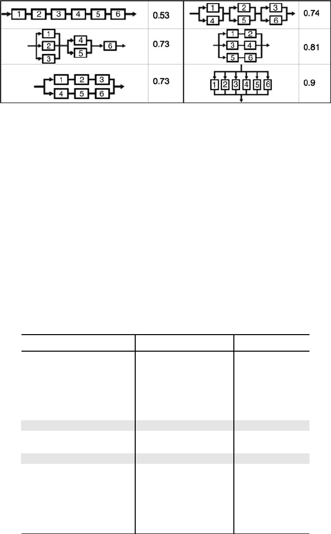
For example, if all machines in a synchronous serial line have the same reliability

R ¼ 0.9, and the line does not have buffers, the system reliability (i.e., % throughput)

as a function of the number of machines in the line N is given in the table below.

N ¼ 1 N ¼ 2 N ¼ 3 N ¼ 4 N ¼ 5 N ¼ 6 N ¼ 7 N ¼ 8 N ¼ 9

0.9 0.81 0.73 0.66 0.59 0.53 0.48 0.43 0.39

With six (6) machines, for example, the theoretical system throughput is only 53%.

Asynchronous serial lines throughput is higher than in the table above, and depends

not only on the ratio MTBF/MTTR but also on the ratio between the cycle time (CT)

and MTBF. The line throughput values were calculated by the ERC/RMS software

PAMS for a perfectly balanced line (and no buffers) for a cycle time CT ¼ 10 minutes,

and are given in the table below.

MTBF MTTR N ¼ 1 N ¼ 2 N ¼ 3 N ¼ 4 N ¼ 5 N ¼ 6 N ¼ 7 N ¼ 8 N ¼ 9

0.9 0.1 0.9 0.893 0.890 0.888 0.887 0.886 0.886 0.885 0.885

9 1 0.9 0.859 0.835 0.820 0.810 0.803 0.797 0.793 0.790

90 10 0.9 0.826 0.767 0.721 0.683 0.651 0.625 0.604 0.585

900 100 0.9 0.819 0.751 0.696 0.645 0.606 0.570 0.539 0.511

The reason for the different values in the two tables is that in the asynchronous

line when one machine fails the other machin es in the line continue to operate, and the

line operation does not stop completely, as assumed by Eq. (10.9). Even when a

machine completed the task it holds the part, so it is acting as a temporary buffer,

which increases the practical throughput of the line. When MTBF  CT, the results

are closer to those obtained by Eq. (10.9).

The parallel system expected throughput is obtained by adding the weighted

reliabilities of the two machines:

EP½¼1

þ 0:5

1R

ðÞþ0:5

1R

ðÞ

þ 0

1R

ðÞ1R

ðÞ¼0:5R

þ 0:5R

ð10:11Þ

IMPACT OF CONFIGURATION ON PERFORMANCE 271

For three machines in parallel the equation is R

/3 þ R

/3. Similar

equations are valid for multiple machines in parallel.

Based on the above table, for R ¼ 0.9, the expected throughput of the six

conﬁgurations in Figure 10.19 was calculated and is given in Figure 10.22 (the

method of calculating the throughput of conﬁguration d, 0.74, is explained below).

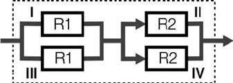
10.5.2.1 Calculating the E xpected Throughput In Conﬁgurations With Cross-

over Calculating the expected throughput in conﬁgurations with crossover requires

building a binary map with all the possible cases. We will show one example of

calculating the expected throughput of the crossover conﬁguration in Figure 10.23.

Each machine can be either up (Up) or down (blank in the table below). For four

machines there are 2

¼ 16 states. The probabilities and the expected throughputs

are in the table below. Note that if machines I and III are both down, or if m achines

II and IV are both down, the system output is 0 (namely, zero expected throughput,

E[P]).

I II III IV Probability Exp. Throughput

Up Up Up Up R

Up Up Up R

(1  R

) 0.5

Up Up Up R

(1  R

0.5

Up Up R

(1  R

)(1  R

) 0.5

Up Up Up R

(1  R

0.5

Up Up 0

Up Up R

(1  R

)(1  R

0.5

Up 0

Up Up Up (1  R

0.5

Up Up (1  R

(1  R

) 0.5

Up Up 0

Up 0

Up Up (1  R

)(1  R

0.5

Up 0

Figure 10.22 The expected throughput of the conﬁgurations in Figure 10.19.

272

SYSTEM CONFIGURATION ANALYSIS

E½P¼R

þ 0:5fR

ð1R

ÞþR

ð1R

ÞR

þ R

ð1R

Þð1R

ÞþR

ð1R

ÞR

þð1R

ÞR

þð1R

Þð1R

ÞR

þ R

ð1R

Þð1R

ÞR

þð1R

ÞR

ð1R

Þg ¼ R

þ R

ð1R

Þð1R

The productivity gain by using the crossover is {R

(1  R

)(1  R

)}.For

R ¼ 0.9 the gain is 0.0081; for R ¼ 0.6 the gain is 0.05764.

To calculate the crossover gain there is no need to calculate the whole table; it is

enough to calculate only the terms that contribute to the throughput gain, and add them

to a calculation performed by using Eqs (10.9) and (10.11).

10.5.3 Comparison of Assembly Systems

Automobile underbodies are assembled by welding operations. The assembly process

is as follows: (1) Incoming parts are located using a ﬁxture. (2) Clamps force two parts

together; then they are welded in speciﬁed locations. (3) Once the welds have been

made, the clamps are released and the part springs back.

Traditional assembly systems for automotive underbodies have been designed

using serial lines. Each station in the line carries out some welds, and the part is sent to

the next station where addi tional welds are done, and so on until completion.

However, advancements in controls have allowed for the implementation of alter-

native system conﬁgurations. Hu and Stecke

conducted a thorough comparison of

four assembly systems, each composed of four stations: a serial line, a system with

four stations in parallel, two parallel lines (two stations in each line), and an RMS

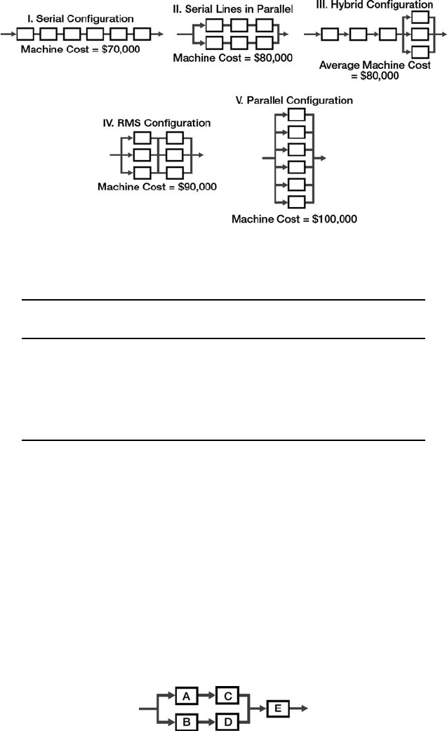
conﬁguration (Figure 10.23). The comparison was done for (1) expected relative

throughput (i.e., productivity) and (2) quality, which was deﬁned as dimensional

accuracy. For the productivity analysis, the reliabilities of the four stations were

assumed to be RA ¼ 0.95, RB ¼ 0.90, RC ¼ 0.93, and RD ¼ 0.98. They found that the

traditional serial assembly line has the worst performance for both productivity and

quality. By contrast, the parallel conﬁguration almost always produced a lower mean

deviation than the serial line, but at the cost of higher six-sigma variation (see

Figure 10.21). The numerical results of the comparison are shown in Table 10.3.

In each column in Table 10.3 we highlighted the best and second best performers.

The results clearly show that serial system of four stations connected in series has by

far the lowest throughput. When the four stations are in parallel, the throughput is the

Figure 10.23 Conﬁguration with crossover connection.

IMPACT OF CONFIGURATION ON PERFORMANCE 273

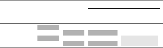
TABLE 10.3 Performance of Four Conﬁgurations

Quality

System

Conﬁguration

Station

Complexity

Relative

Throughput

Mean

Deviation (mm)

6 Sigma of

Audited Point (mm)

Serial Low 0.779 18.40 56.68

Parallel High 0.940 14.40 59.97

Parallel lines Medium 0.884 15.85 55.36

RMS conﬁguration Medium 0.886 14.84 55.45

highest. The RMS conﬁguration has a slightly higher throughput than the two parallel-

line conﬁguration. In general, the greater the number of possible material ﬂow paths a

system has, the greater its throughput. For example, a serial system has only one ﬂow

path, so the system shuts down if only one machine fails. A parallel-line system offers

much more redundancy than a serial system, and therefore exhibits a great increase in

throughput. The RMS conﬁguration has four ﬂow paths and yields improved

throughput.

Nevertheless, in the parallel conﬁguration all the assembly tasks must be done at

each station. When assembling a complex product, the number of tools and number of

components to be assembled is large, the process becomes too complex, and typically

it is impossible to ever act ually reach the theoretical maximum throughput.

10.5.4 Capacity Scalability

To adapt to ﬂuctuations in product demand, capacity must be adjusted quickly and

cost-effectively. Capacity scalability is the ability to rapidly adjust the production

capacity of a system in discrete steps. Even though a system will be reconﬁgured many

times, the initial conﬁguration has a profound effect on the system’s adjustment step-

size and its cost. For example, if a serial line (Fig. 10.19a) needs to increase its

production capacity to satisfy market demand, an entire new line has to be added. The

step-size of this addition exactly doubl es the production capacity of the system. This

addition will be expensive, since there is no guarantee that the extra capacity will ever

be fully utilized, risking a substantial ﬁnancial loss.

System scalability was deﬁned in Chapter 6 as

System scalabili ty ¼ 100 smallest incremental capacity in percentage

Scalability is indicated as the capacity increment by which the system can be

adjusted to meet new market demand. The serial line has a minimum production

capacity increment of 100% of the system; we deﬁne it as scalability ¼ 100  100

¼ 0%. The conﬁguration in Figure 10.19c has a scalability of 50% and that of

Fig. 10.19e has a scalability of 67%.

The smallest adjustment steps can be done when the original system is purely

parallel (e.g., Figure 10.19f). However, the initial cost of a parallel system is the

highest. In parallel conﬁgurations each machine must duplicate all operations on the

product, and therefore each machine must have more tools and be able to perform

274 SYSTEM CONFIGURATION ANALYSIS

more functions. As a result, the cost per additional volume increment is the highe st

with parallel conﬁgurations.

The conﬁguration depicted in Fig. 10.19e (two stages; three machines per stage)

might be a com promise. In this case, for example, if a product requires machining on

both the upper and side surfaces, Machines 1,3, and 5 might be three-axis vertical

milling machines, and Machines 2, 4, and 6 might be three-axis horizontal milling

machines. Conversely, in a parallel system, all six mac hines in Fig. 10.19f must be

ﬁve-axis milling machines—a system that is much more expensive. The drawback

of the syst em in Fig. 10.17e is that capacity scalability must be performed in steps of

33.3% rather than steps of 16.6% as with the parallel conﬁguration.

The steps of adding capacity in the conﬁgurations of Figures 10.19c and 10.19d are

even bigger—50%. Figure 10.19b represents a case in which the steps are unequal: an

additional 33.3% capacity requires three machines of type 1, 4, and 6; but the next

additional increase of 16.6% requires adding only one machine of type 1, and so that

increment is not expensive. This conﬁguration might best be applied in cases where

Machine 6 performs a brief but specialized operation such as laser welding.

Of course, theoretically, the manufacturer can always add one machine in parallel

(a machine that does the whole part processing), to any existing conﬁguration; making

the addition an equal match for all conﬁgurations. However, this is not recommended

in practice, since integration of an exceptional and complex machine into a system

that does not otherwise include such machines increases the integration and main-

tenance costs, and may cause problems in achieving the required part quality.

To compare the six conﬁgurations in Figure 10.19, we made cost assumptions

summarized in Table 10.4, where the base cost of the machines are all the same,

$100,000. But because of the different number of operations required with each

machine, the tool magazine capacity and the tooling cost are varied. When we add the

scalability cost and its smallest possible increments into the calculation, it becomes

evident that Conﬁguration d is preferred. (We have not done scalability analysis for

Conﬁguration b because it is a special case in which the processing time on each

machine at the ﬁrst stage is three times larger than that in the last stage.)

The following example clariﬁes the option of adding small incremental capacity

steps in Conﬁguration d in Figure 10.19.

Example: Processing a given part requires 21 machining operations of 30 seconds

each (totaling 630 seconds, or 10.5 minutes, needed to machine each part). The

required demand is 274 parts per 8-hour shift (480 minutes) . Therefore, the required

cycle time is 1.75 minutes/part.

(a) Design a scalable system conﬁguration.

(b) After 1 year, the demand has grown, and 320 parts per shift are needed (i.e.,

reducing the cycle time to 1.5 minutes/part). How many machines should be

added, and what is the new conﬁguration?

According to Eq. (10.1) six machines are needed: 274  10.5/480 ¼ 6. Although

the least expensive initial conﬁguration is six machines in a serial transfer line, the

preferred solution is the RMS conﬁguration shown in Figure 10.24, in which each

machine does seven operations (210 seconds per machine). When the demand grows

IMPACT OF CONFIGURATION ON PERFORMANCE 275

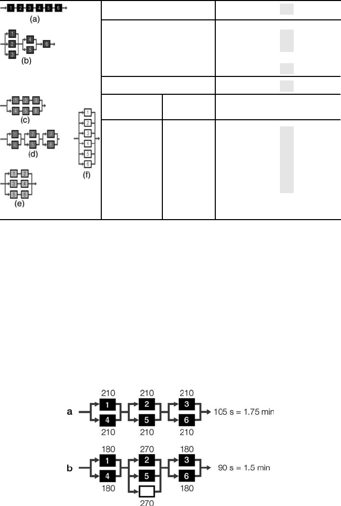
to 320 parts/day, according to Eq. (10.1), seven machines are neede d. Only this

selected RMS conﬁguration yields the optimal solution—adding one machine to

Stage 2. One operation is shifted from Stage 1 to Stage 2 (so each machine in Stage

1 operates for 180 seconds), and another operation is shifted from Stage 3 to Stage

2 (so each machine in Stage 2 operates for 270 seconds).

The initial capital investment in the RMS conﬁguration is a bit higher than that in

a serial line, but the extra investment is like buying insurance for a future event that is

likely to occur. If the event does happen, the system can be easily scaled up and the

new demand can be supplied at the minimum additional investment. If the demand is

unchanged, a small capital investment (on a more sophisticated material handling

system) was lost.

Figure 10.24 When demand grows, the initial system a is cost-effectively scaled up to

conﬁguration b to meet the new demand.

TABLE 10.4 Initial System Cost and Cost of Scalability (in $1000)

Conﬁguration a b c d e f

Cost of six machines 600 600 600 600 600 600

Tooling cost per machine 5 20 20 20 25 42

Material handling cost 100 150 120 150 156 162

Total initial system cost 730 870 840 870 906 1,014

Add machines Add Volume Scalability Cost

One 16.6 – – 145 – 169

Two 33.3 – – 290 302 338

Three 50.0 – 420 435 – 507

Four 66.7 – – 580 604 676

Five 83.3 – – 725 – 845

Six 100.0 730 870 840 870 906 1,014

276 SYSTEM CONFIGURATION ANALYSIS

10.5.5 Selecting a System Conﬁgur ation

As we have said before, in selecting the most appropriate conﬁguration of a

production system the designer has to take into account several considerations:

Initial investment cost

Expected throughput with reliability less than 100%

Scalability—the increment of production capacity gained by adding one ma-

chine, or a minimum number of machines

Quality—capability of the system in producing parts with minimal variation

Number of product variations that the system can produce

Floor space.

Calculating the system’s expected throughput with reliability less than 100% is

more tedious than just using the reliability equations. This is because the equations

assume a perfectly balanced system, but in reality systems are not balanced. Let us

calculate, for example, the throughput for the conﬁguration in Figure 10.16 with

machine reliability of 98%.

To have any throughput , Machines 3, 4, and 5 must operate. Only the cases that are

in the table below (with Machines 3, 4, 5 up) will yield any production. Note, for

example, that if Machine 1 is down, the bottleneck moves from Machine 4 to Machine

2 and the new cycle time for that stage is 3.7 minutes (and not 1.85 minutes). The

throughput is the total of the right column in the table—454.8 parts per day (rather

than 500 with 100% reliability). For this conﬁguration a reduction of 2% in machine

reliability caused a reduction of 9% in the system throughput.

A. Case

B. Event

Probability

C. New

Cycle

Time

Throughput

B  D ¼

Adjusted

Throughput

1,2,6,7 up 0.868 2 500.0 434.1

1 or 2 up; 6 and 7 up 0.035 3.7 270.3 9.6

1 and 2 up; 6 or 7 up 0.035 3.3 303.0 10.7

1 or 2 up; 6 or 7 up 0.001 3.7 270.3 0.4

For the example in Section 10.4 the throughputs with reliabilities of 0,98, 0.95, and

0.9 were calculated, as well as the scalable throughputs, and they are given in

Table 10.5.

The ranking to determine the most appropriate conﬁguration is subjective and

depends on the weight that the designer (and company) assigns to each factor

(cost, scalability, etc). In our opinion, the conﬁguration that the designer would

most likely favor (Rank ¼ 1) is the one shown in Figure 10.14B (on the right). The

throughput requirement (500 parts/day) is met with machine reliability of 98%

IMPACT OF CONFIGURATION ON PERFORMANCE 277

(or better). This conﬁguration has a good scalability and reasonable investment

cost.

Remember, a serial system is ranked lowest when considering scalability, con-

vertibility and expected throughput with reliability less than 100%. These are the

main reasons for not recommending serial transfer lines when demand is uncertain.

The more that a system moves from serial toward parallel conﬁguration, the better that

it ranks on these three categories.

However, as a system moves toward parallel

conﬁgurations, the system becomes more expensive. The initial cost of purely parallel

systems is very high.

It has been shown in this section that the conﬁguration of a system has a profound

effect on the performance of the system , including productivity, capacity scalability,

and part quality. These features also inﬂuence the life-cycle cost of the manufacturing

system. This text offers the system designer analytical tools to aid in the selection of

the appropriate system conﬁguration. Although the examples given above are from

the machining domain, the methodology may be applied to other man ufacturing

domains as well.

PROBLEMS

10.1 A manufacturing system has to produce three products daily in the quantities

given in the table below. Each product requires six manufacturing tasks to be

completed. The sequence of the tasks must be done in the order given in the

table (i.e., task 1 then 2, then 3, etc.). We assume 1000 minutes per working

day.

The manufacturing time in minutes for each task for each product is given in

the following table:

TABLE 10.5 Comparison of Eight Conﬁgurations in the Example

Scalability

Throughput Throughput

Conﬁg.

in Fig.

Stages

Throughput

at R ¼ 100%

N ¼ 7

Machines

With

N ¼ 8

With

N ¼ 9 R ¼ 98% R ¼ 95% R ¼ 90% Cost RANK

10.15 5 500 540 588 455 393 306 Low 7

10.14A 4 540 540 606 500 446 338 Med 6

10.14B 4 540 571 606 500 446 371 Med 5

10.14C 4 500 540 588 467 419 348 Med 8

10.13A 3 540 540 625 512 473 415 Med 2

10.13B 3 540 578 606 511 472 414 Med 1

10.13C 3 540 588 588 511 470 406 Med 4

10.12 2 540 588 705 522 497 455 High 3

Gray background ¼ ‘

Best;

; light gray background ¼ very good result compared with alternatives.

278 SYSTEM CONFIGURATION ANALYSIS

Product A Product B Product C

Daily Quantity 200 150 150

Task #1 1.5 1.5 1.5

Task #2 1.5 1.5 1.5

Task #3 1.5 1.5 1.5

Task #4 2 1.5 2

Task #5 1 2 2

Task #6 1 1.5 2

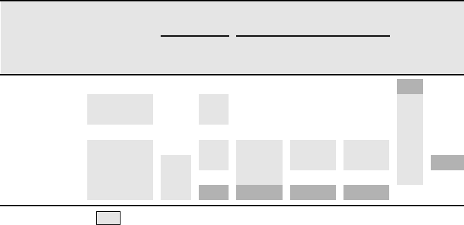
The cost of the various machines is given in Figure 10.25. The cost of the

material handling system for System I is $120,000; for syst ems II & III—

$200,000; for systems IV & V—$250,000. Assuming that the equipment

reliability is 100%, compare the ﬁve conﬁgurations in Figure 10.25 in terms of

(1) investment cost (quantitative results); (2) productivity (qualitative anal-

ysis); and (3) producing three produc ts simultaneously (qualitative analysis).

10.2 In the conﬁguration depicted in Figure 10.26, you have to place ﬁve machines

that have the following reliabilities: I ¼ 0.5, II ¼ 0.6, III ¼ 0.7, IV ¼ 0.8, and

V ¼ 0.9.

Figure 10.25 Five conﬁgurations of Problem 10.1.

Figure 10.26 Two conﬁgurations.

PROBLEMS 279

(a) Calculate the expected throughput if A ¼ I, B ¼ II, C ¼ III, D ¼ IV, and

E ¼ V.

(b) Place the machines such that the system expected throughput is maximized

(calculate it).

stages, with higher expected throughput? What is the reason that the

conﬁguration(s) have higher throughput?

(d) Can you draw a conclusion about planning similar conﬁgurations?

10.3 In the conﬁguration in Figure 10.23 the following machine reliabilities are

given: I ¼ 0.5, II ¼ 0.6, III ¼ 0.7, and IV ¼ 0.8. Calculate the system expected

throughput. Is there another placement of the machines that will increas e the

system throughput?

10.4 In the conﬁguration depicted in Figure 10.23 the part is machined in two

operations. In the ﬁrst stage the operation takes 6 minutes per machine, and in

the second stage 5.4 minutes per machine. What is the throughput of the system

in parts/hour?

What is the throughput of the syst em if the reliability of each machine in the

ﬁrst stage is 0.9, and the reliability of each machine in the second stage is 0.8?

REFERENCES

1. Y. Koren, S. J. Hu, and W. T. Weber. Impact of manufacturing system conﬁguration on

performance. CIRP Annals, 1998, Vol. 47, No. 1, pp. 689–698.

2. S. J. Hu. Stream of variation theory for automotive body assembly. Annals of the CIRP, 1997,

Vol. 46/1, pp. 1–6.

3. W. T. Weber. Impact of manufacturing system conﬁguration on performance. D. Eng.

Thesis, University of Michigan, 1997.

4. T. Faricy. Reliability and Maintainability. Society of Manufacturing Engineers (SME) and

the National Center for Manufacturing Sciences (NCMS), 1993.

5. S. J. Hu and K. E. Stecke. Analysis of various assembly system conﬁgurations for quality

and productivity. International Journal of Manufacturing Research, July 2009, Vol. 4, No. 3,

pp. 281–305.

6. V. Maier-Speredelozzi, Y. Koren, and S.J. Hu. Convertibility measures for manufacturing

systems. CIRP Annals, August 2003, Vol. 52, No. 1, pp. 367–371.

280

SYSTEM CONFIGURATION ANALYSIS