Korb K.B., Nicholson A.E. Bayesian Artificial Intelligence

Подождите немного. Документ загружается.

We have also described in some detail the development of BN models for three

quite different applications. First, we described a game playing application, poker,

where the BN was used to estimate the probability of winning and to make betting

decisions. Then we saw that a DBN model for ambulation monitoring and fall di-

agnosis can overcome the limitations of a state-machine approach. Given evidence

from sensor observations, the DBN outputs beliefs about the current walking status

and makes predictions regarding future falls. The model represents sensor error and

is parameterized to allow customization to the individual being monitored. Finally,

we looked at how BNs can be used simultaneously for normative domain modeling

and user modeling in NAG, by integrating them with semantic networks using an

attentional process.

At this stage, it is also worth noting that different evaluation methods were used

in each of the example applications, including an experimental/empirical evaluation

for the Bayesian poker player, and case-based evaluation for ambulation monitoring

DBN. We take up the issue of evaluation in Chapter 10.

5.7 Bibliographic notes

There have been a number of attempts to collect information about successful BN

applications and, in particular, systems in regular use, such as that of Russ Greiner

(

http://excalibur.brc.uconn.edu/ baynet/fieldedSystems.html)

and Eugene Santos Jr. These and others have been used as a basis for our survey

5.2.

An interesting case study of PATHFINDER’s developmentis given in [237, p. 457].

The high level of interest in BN applications for medicine is indicated by the work-

shop Bayesian Models in Medicine at th

e 2001 European Conference on AI in Med-

icine (AIME’01). The journal Artiﬁcial Intelligence in Medicine may also be con-

sulted. Husmeier et al. have a forthcoming text on probabilistic models for medical

informatics and bioinformatics [119].

Findler [82] was the ﬁrst to work on automated poker play, using a combination

of a probabilistic assessment of hand strength with the collection of frequency data

for opponent behavior to support the reﬁnement of the models of opponent. Water-

man [295] and Smith [259] used poker as a testbed for automatic learning methods,

speciﬁcally the acquisition of problem-solving heuristics through experience. Koller

and Pfeffer [152] have developed Gala, a system for automating game-theoretic anal-

ysis for two-player competitive imperfect information games, including simpliﬁed

poker. Although they use comparatively efﬁcient algorithms, the size of the game

tree is too large for this approach to be applied to full poker. Most recently, Billings

et al. [19, 20] have investigated the automation of the poker game Texas Hold’em

with their program Poki. Our work on Bayesian networks for poker has largely ap-

peared in unpublished honors theses (e.g., [132, 38]), but see also [160].

Ambulation monitoring and fall detection is an ongoing project, with variations,

extensions and implementations described in [203, 186, 300].

NAG has been described in a sequence of research articles, including the ﬁrst

description of the architecture [305], detailed architectural descriptions (e.g., [306]),

a treatment of issues in the presentation of arguments [228] and the representation of

human cognitive error in the user model [136].

5.8 Problems

Problems using the example applications

Problem 1

Build the normative asteroid Bayesian network of Figure 5.10 and put in some likely

prior probabilities and CPTs. Make a copy of this network, but increase the prior

probability for P4; this will play the role of the user model for this problem. Operate

both networks by observing P1, P2 and P3, reporting the posterior belief in P4 and

This is not the way that NAG operates. Explain how it differs. In your work has

“explaining away” played a role? Does it in the way NAG dealt with this example in

the text? Explain your answer.

Problem 2

What are the observation nodes when using the Poker network for estimating BPP’s

probability of winning? What are the observation nodes when using the network to

assess the opponent’s estimate of winning chances?

Problem 3

Determine a method of estimating the expected future contributions to the pot by

both BPP and OPP, to be used in the utilities in the Winnings node. Explain your

method together with any assumptions used.

Problem 4

All versions of the Bayesian Poker Player to date have used a succession of four

distinct Bayesian networks, one per round. In a DDN model for poker, each round in

the poker betting would correspond to a single time slice in the DDN, which would

allow explicit representation of the interrelation between rounds of play.

1. How would the network structure within a single time slice differ from the DN

shown in Figure 5.5?

2. What would the interslice connections be?

3. What information and precedence links should be included?

Problem 5

5.4.4, we saw how the use of a sensor status node can be used to model both

intermittent and persistent faults in the sensor. In the text this node had only two

states, working and defective, which does not represent the different kinds of faults

that may occur, in terms of false negatives, false positives, and so on. Redesign the

sensor status modeling to handle this level of detail.

New Applications

The BN, DBN and decision networks surveyed in this chapter have been developed

over a period of months or years. It is obviously not feasible to set problems of a

similar scope. The following problems are intended to take 6 to 8 hours and require

domain knowledge to be obtained either from a domain expert or other sources.

Problem 6

Suppose that a dentist wants to use a Bayesian network to support the diagnosis and

treatment of a patient’s toothache. Build a BN model including at least 3 possible

causes of toothache, any other symptoms of these causes and two diagnostic tests.

Then extend the model to include possible treatment options, and a utility model that

includes both monetary cost and less tangible features such as patient discomfort and

health outcomes.

Problem 7

Design a heart attack Bayesian network which can be used to predict the impact of

changes in lifestyle (e.g., smoking, exercise, weight control) on the probability of

premature death due to heart attack. You will have to make various choices about

the resolution of your variables, for example, whether to model years or decades of

life lost due to heart attack. Such choices may be guided by what data you are able

to ﬁnd for parameterizing your network. In any case, do the best you can within the

time frame for the problem. Then use your network to perform a few case studies.

Estimate the expected number of years lost from heart attack. Then model one or

more lifestyle changes and re-estimate.

Problem 8

Build a Bayesian network for diagnosing why a car on the road has broken down.

First, identify the most important ﬁve or six causes for car breakdown (perhaps, lack

of fuel or the battery being ﬂat when attempting to restart). Identify some likely

symptoms you can use to distinguish between these different causes. Next you need

the numbers. Do the best you can to ﬁnd appropriate numbers within the time frame

of the assignment, whether from magazines, the Internet or a mechanic. Run some

different scenarios with your model, reporting the results.

Problem 9

Design a Bayesian network bank loan credit system which takes as input details

about the customer (banking history, income, years in job, etc.) and details of a pro-

posed loan to the customer (type of loan, interest rate, payment amount per month,

etc.) and estimates the probability of a loan default over the life of a loan. In order to

parameterize this network you will probably have to make guestimates based upon

aggregate statistics about default rates for different segments of your community,

since banks are unlikely to release their proprietary data about such things.

Part II

LEARNING CAUSAL

MODELS

These three chapters describe how to apply machine learning to the task of learn-

ing causal models (Bayesian networks) from statistical data. This has become a hot

topic in the data mining community. Modern databases are often so large they are im-

possible to make sense of without some kind of automated assistance. Data mining

aims to render that assistance by discovering patterns in these very large databases

and so making them intelligible to human decision makers and planners. Much of

the activity in data mining concerns rapid learning of simple association rules which

may assist us in predicting a target variable’s value from some set of observations.

But many of these associations are best understood as deriving from causal relations,

hence the interest in automated causal learning, or causal discovery.

The machine learning algorithms we will examine here work best when they have

large samples to learn from. This is just what large databases are: each row in

a relational database of N columns is a joint observation across N variables. The

number of rows is the sample size.

In machine learning samples are typically divided into two sets from the begin-

ning: a training set and a test set. The training set is given to the machine learning

algorithm so that it will learn whatever representation is most appropriate for the

problem; here that means either learning the causal structure (the dag of a Bayesian

network) or learning the parameters for such a structure (e.g., CPTs). Once such a

representation has been learned, it can be used to predict the values of target vari-

ables. This might be done to test how good a representation it is for the domain.

But if we test the model using the very same data employed to learn it in the ﬁrst

place, we will reward models which happen to ﬁt noise in the original data. This is

called overﬁtting. Since overﬁtting almost always leads to inaccurate modeling and

prediction when dealing with new cases, it is to be avoided. Hence, the test set is

isolated from the learning process and is used strictly for testing after learning has

completed.

Almost all work in causal discovery has been looking at learning from observa-

tional data — that is, simultaneous observations of the values of the variables in the

network. There has also been work on how to deal with joint observations where

some values are missing, which we discuss in Chapter 7. And there has been some

work on how to infer latent structure, meaning causal structure involving variables

that have not been observed (also called hidden variables). That topic is beyond the

scope of this text (see [200] for a discussion). Another relatively unexplored topic is

how to learn from experimental data. Experimental data report observations under

some set of causal interventions; equivalently, they report joint observations over the

augmented models of

3.8, where the additional nodes report causal interventions.

The primary focus of Part II of this book will be the presentation of methods that are

relatively well understood, namely causal discovery with observational data. That is

already a difﬁcult problem involving two parts: searching through the causal model

space

, looking for individual (causal) Bayesian networks to evaluate; eval-

uating each such

relative to the data, perhaps using some score or metric, as in

Chapter 8. Both parts are hard. The model space, in particular, is exponential in the

number of variables (

6.2.3).

We present these causal discovery methods in the following way. We start in Chap-

ter 6 by describing algorithms for the discovery of linear causal models (also called

path models, structural equation models). We begin with them for two reasons. First,

this is the historical origin of graphical modeling and we think it is appropriate to pay

our respects to those who invented the concepts underlying current algorithms —

particularly since they are not very widely known in the AI community. Those who

have a background in the social sciences and biology will already be familiar with

the techniques. Second, in the linear domain the mathematics required is particularly

simple, and so serves as a good introduction to the area. It is in this context that we

introduce constraint-based learning of causal structure: that is, applying knowl-

edge of conditional independencies to make inferences about what causal relation-

ships are possible. In Chapter 7 we consider the learning of conditional probability

distributions from sample data. We start with the simplest case of a binomial root

node and build to multinomial nodes with any number of parents. We then discuss

learning parameters when the data have missing values, as is normal in real-world

problems. In dealing with this problem we introduce expectation maximization

(EM) techniques and Gibbs sampling. In the ﬁnal chapter of this part, Chapter 8,

we introduce the metric learning of causal structure for discrete models, including

our own, CaMML. Metric learners search through the exponentially complex space

of causal structures, attempting to ﬁnd that structure which optimizes their metric.

The metric usually combines two scores, one rewarding ﬁt to the data and the other

penalizing overly complex causal structure.

Learning Linear Causal Models

6.1 Introduction

Thus far, we have seen that Bayesian networks are a powerful method for represent-

ing and reasoning with uncertainty, one which demonstrably supports normatively

correct Bayesian reasoning and which is sufﬁciently ﬂexible to support user model-

ing equally well when users are less than normative. BNs have been applied to a very

large variety of problems; most of these applications have been academic exercises

— that is to say, prototypes intended to demonstrate the potential of the technology,

rather than applications that real businesses or government agencies would be rely-

ing upon. The main reason why BNs have not yet been deployed in many signiﬁcant

industrial-strength applications is the same reason earlier rule-based expert systems

were not widely successful: the knowledge bottleneck.

Whether expert systems encode domain knowledge in rules or in conditional prob-

ability relations, that domain knowledge must come from somewhere. The main

plausible source until recently has been human domain experts. When building

knowledge representations from human experts, AI practitioners (called knowledge

engineers in this role) must elicit the knowledge from the human experts, interview-

ing or testing them so as to discover compact representations of their understanding.

This encounters a number of difﬁculties, which collectively make up the “knowledge

bottleneck” (cf. [81]). For example, in many cases there simply are no human ex-

perts to interview; many tasks to which we would like to put robots and computers

concern domains in which humans have had no opportunity to develop expertise —

most obviously in exploration tasks, such as exploring volcanoes or exploring sea

bottoms. In other cases it is difﬁcult to articulate the humans’ expertise; for exam-

ple, every serious computer chess project has had human advisors, but human chess

expertise is notoriously inarticulable, so no good chess program relies upon rules

derived from human experts as its primary means of play — they all rely upon brute-

force search instead. In all substantial applications the elicitation of knowledge from

human experts is time consuming, error prone and expensive. It may nevertheless be

an important means of developing some applications, but if it is the only means, then

the spread of the underlying technology through any large range of serious applica-

tions will be bound to be slow and arduous.

The obvious alternative to relying entirely upon knowledge elicitation is to employ

machine learning algorithms to automate the process of constructing knowledge rep-

resentations for different domains. With the demonstrated potential of Bayesian net-

works, interest in methods for automating their construction has grown enormously

in recent years. In this chapter we look again at the relation between conditional

independence and causality, as this provides a key to causal learning from observa-

tional data.

This key relates to Hans Reichenbach’s work on causality in The Direction of

Time (1956) [233]. Recall from

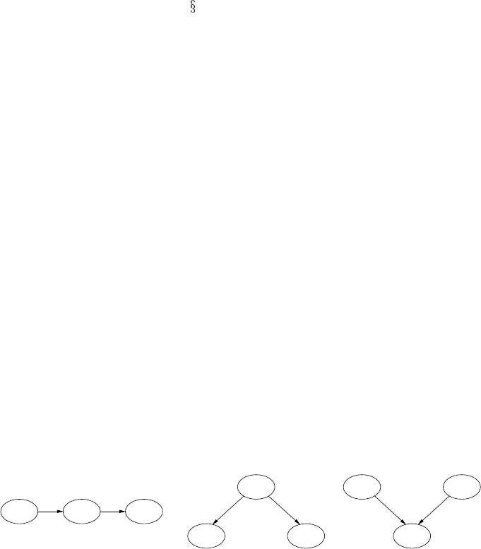
2.4.4 the types of causal structures available for

three variables that are in an undirected chain; these are causal chains, common

causes and common effects, as in Figure 6.1. Reichenbach proposed the following

principle:

Conjecture 6.1 Principle of the Common Cause If two variables are probabilisti-

cally dependent, then either one causes the other (directly or indirectly) or they have

a common ancestor.

Reichenbach also attempted to analyze time and causality in terms of the differ-

ent dependency structures exempliﬁed in Figure 6.1; in particular, he attempted to

account for time asymmetry by reference to the dependency asymmetry between

common causal structures and common effect structures. In this way he anticipated

d-separation, since that concept depends directly upon the dependency asymmetries

Reichenbach studied. But it is the Principle of the Common Cause which under-

lies causal discovery in general. That principle, in essence, simply asserts that be-

hind every probabilistic dependency is an explanatory causal dependency. And that

is something which all of science assumes. Indeed, we should likely abandon the

search for an explanatory cause for a dependency only after an exhaustive and ex-

hausting search for such a cause had failed — or, perhaps, if there is an impossibility

proof for the existence of such a cause (as is arguably the case for the entangled

systems of quantum mechanics). The causal discovery algorithms of this chapter

explicitly search for causal structures to explain probabilistic dependencies and, so,

implicitly pay homage to Reichenbach.

(b) (c)

(a)

CBA

FIGURE 6.1

(a) Causal chain; (b) common cause; (c) common effect.

6.2 Path models

The use of graphical models to represent and reason about uncertain causal relation-

ships began with the work of the early twentieth-century biologist and statistician

Sewall Wright [302, 303]. Wright developed graphs for portraying linear causal re-

lationships and parameterized them based upon sample correlations. His approach

came to be called path modeling and has been extensively employed in the social

sciences. Related techniques include structural equation modeling, widely employed

in econometrics, and causal analysis. Behind the widespread adoption of these meth-

ods is, in part, just the restriction to linearity, since linearity allows for simpler math-

ematical and statistical analysis. Some of the restrictiveness of this assumption can

be relaxed by considering transformations of non-linear to linear functions. Never-

theless, it is certain that many non-linear causal relations have been simplistically

understood in linear terms, merely because of the nature of the tools available for

analyzing them.

In using Bayesian networks to represent causal models we impose no such restric-

tions on our subject. Nevertheless, we shall ﬁrst examine Wright’s “method of path

coefﬁcients.” Path modeling is preferable to other linear methods precisely because

it directly employs a graphical approach which relates closely to that of Bayesian

networks and which illustrates in a simpler context many of the causal features of

Bayesian networks.

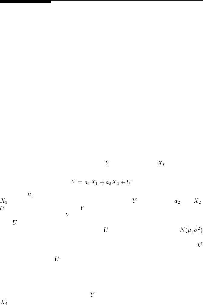
A linear model relates the effect variable

to parent variables via an additive,

linear function, as in:

(6.1)

In this case

is a constant coefﬁcient that reﬂects the extent to which parent variable

inﬂuences, accounts for or explains the value of ; similarly for and .

represents the mean value of and the variation in its values which cannot be

explained by the model. If

is in fact a linear function of all of its parent variables,

then

represents the cumulative linear effect of all the parents that are unknown

or unrepresented in this simple model. If

is distributed as a Gaussian

(normal), the model is known as linear Gaussian. This simple model is equally

well represented by Figure 6.2. Usually, we will not bother to represent the factor

explicitly, especially in our graphical models. When dealing with standardized linear

models, the impact of

can always be computed from the remainder of the model

in any case.

A linear model may come from any source, for example, from someone’s imag-

ination. It may, of course, come from the statistical method of linear regression,

which ﬁnds the linear function which minimizes unpredicted (residual) variation in

the value of the dependent variable

given values for the independent variables

. What we are concerned with in this chapter is the discovery of a joint system

of linear equations by means distinct from linear regression. These means may not

necessarily strictly minimize residual variation, but they will have other virtues, such