Kopnin N.B. Theory of Nonequilibrium Superconductivity

Подождите немного. Документ загружается.

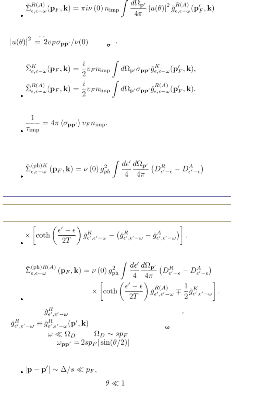
in a complete analogy to eqn (5.69). The impurity self-energy is written in the

Born approximation. The Fourier transformed impurity potential squared is

where

is the scattering cross section. One can

thus present the self-energy as

Remind that the scattering rate in the normal sate is

The phonon self-energy can also be expressed through the quasiclassical

functions. It is

end p.172

The relaxation part of the regular phonon self-energy takes the form

The function in these equations carries the momentum p , i.e.,

. Since the phonon energy is ~ T and satisfies

the inequality

where is the Debye frequency, the

phonon energy is

where s is the velocity of sound.

Because the relative change in the momentum during the emission of a phonon

is small

the the scattering angle of a phonon . We have

PRINTED FROM OXFORD SCHOLARSHIP ONLINE (www.oxfordscholarship.com)

Oxford Scholarship Online: Theory of Nonequilibrium Supe... http://www.oxfordscholarship.com/oso/private/content/phy...

第3页共7页 2010-8-8 15:50

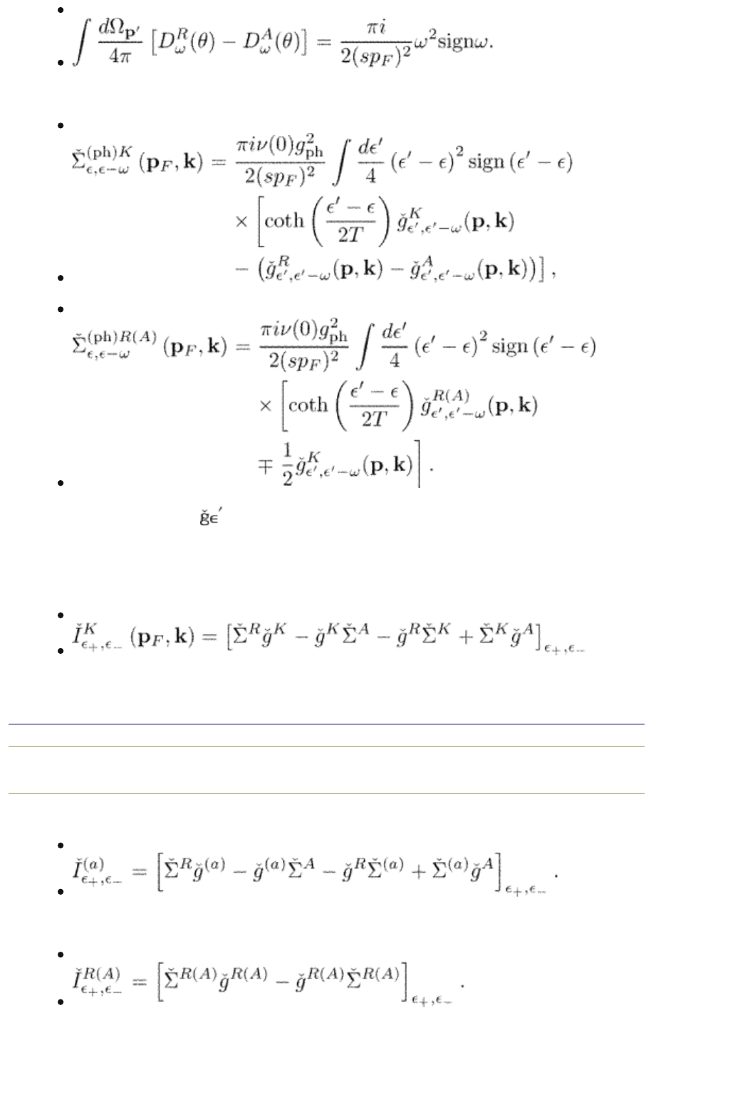
(9.11)

As a result,

(9.12)

(9.13)

Note that the functions (p, r) in eqns (9.12, 9.13) have the same momentum

p as the self-energy itself since the relative change in the momentum during

interaction with the acoustic phonons is small.

The collision integral eqn (9.2) takes the form

(9.14)

where all terms are expressed through quasiclassical functions.

end p.173

The collision integral eqn (9.5) for the anomalous function is

(9.15)

For regular functions in eqn (9.7) we obtain

(9.16)

9.1.2 Order parameter, current, and particle density

PRINTED FROM OXFORD SCHOLARSHIP ONLINE (www.oxfordscholarship.com)

Oxford Scholarship Online: Theory of Nonequilibrium Supe... http://www.oxfordscholarship.com/oso/private/content/phy...

第4页共7页 2010-8-8 15:50

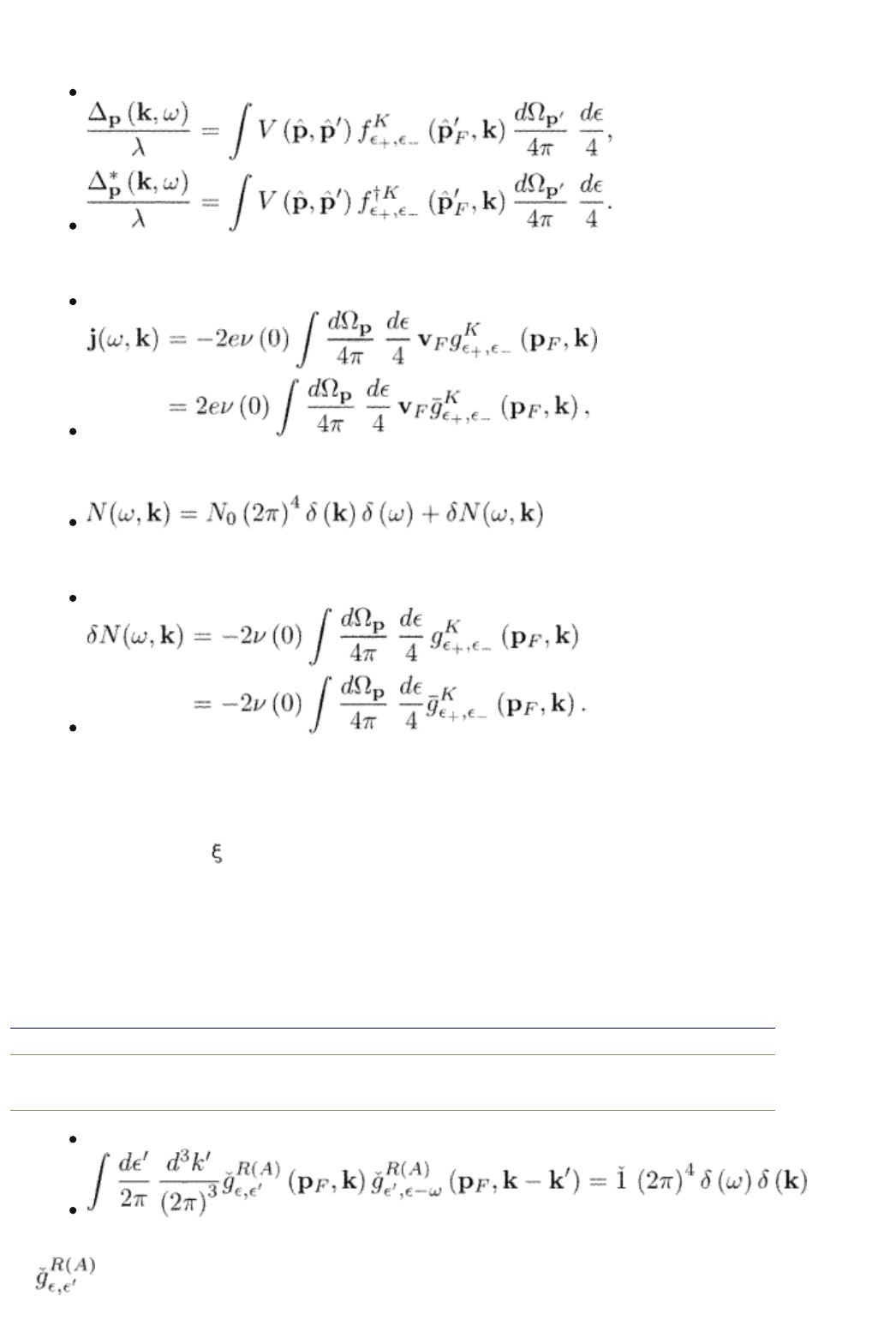
The order parameter, current, and the particle density can be expressed through

the quasiclassical functions in the same way as for the static case. The order

parameter equation becomes for a general pairing

(9.17)

The expression for current is

(9.18)

and the electron density has the form

Where

(9.19)

They are easily obtained from the corresponding equations in terms of the total

Green functions and the quasiclassical expressions derived earlier for the static

case. The diamagnetic term in the current, eqn (9.18), disappears in the

quasiclassical representation since it is canceled by the normal-state contribution

subtracted from the

-integrated function g as it has been shown earlier.

9.1.3 Normalization of the quasiclassical functions

Here we derive useful identities for the total quasiclassical Green functions. First

of all, we demonstrate that the normalization condition

end p.174

(9.20)

holds in the nonstationary case, as well. To see this, we multiply eqn (9.7) by

first from the left and then from the right and add the two equations. We

PRINTED FROM OXFORD SCHOLARSHIP ONLINE (www.oxfordscholarship.com)

Oxford Scholarship Online: Theory of Nonequilibrium Supe... http://www.oxfordscholarship.com/oso/private/content/phy...

第5页共7页 2010-8-8 15:50

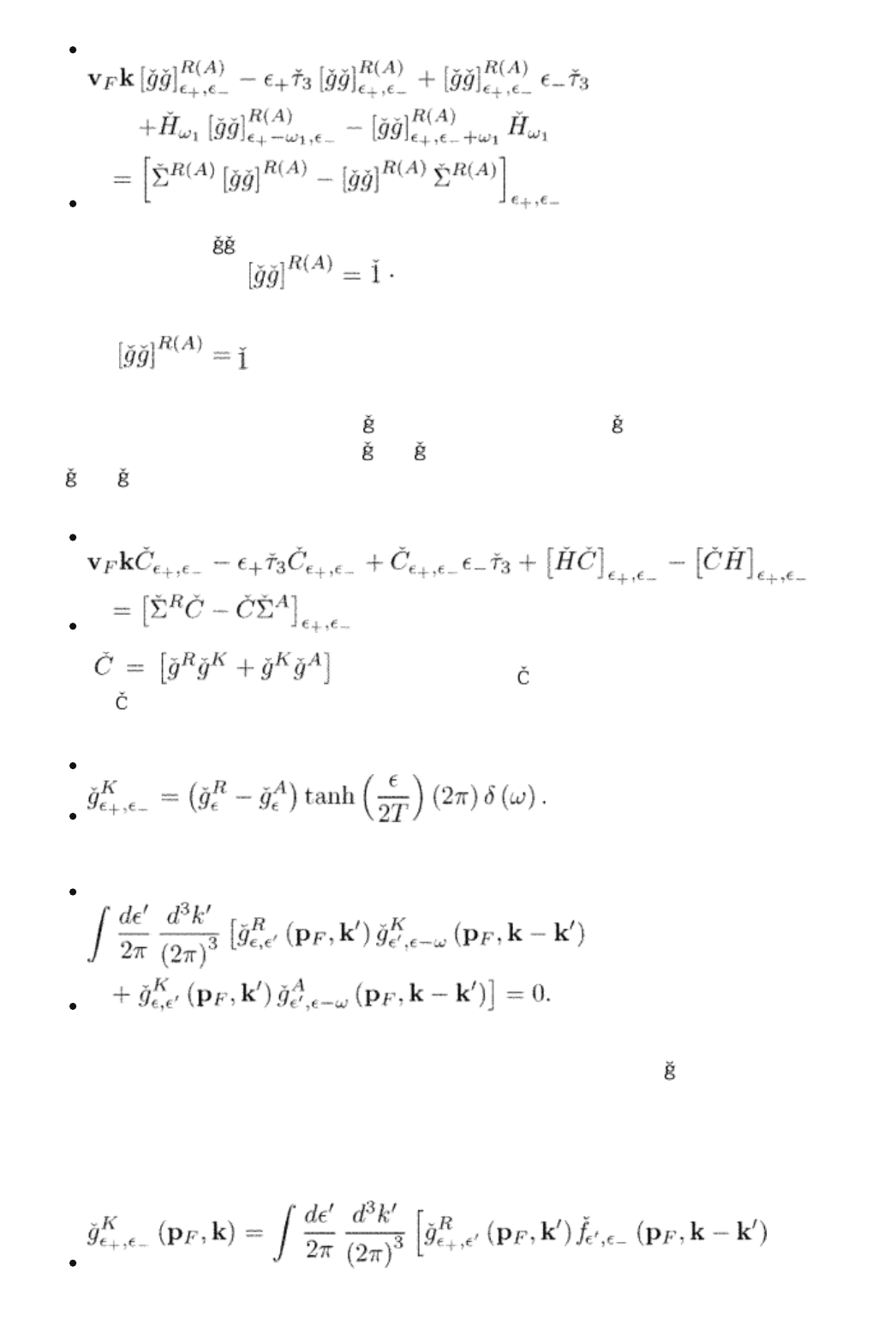
obtain

(9.21)

where the shortcut [ ] again stands for the expression in the l.h.s. of eqn

(9.20). We observe that

const is a solution of eqn (9.21). We

can use the same argumentation as for the static case. We assume that, at large

distances the system is in equilibrium and is homogeneous. Therefore the

condition

, being fulfilled hi equilibrium, should also hold in a

general situation. We thus arrive at eqn (9.20).

Let us now multiply eqn (9.2) first by

from the left and then by

from the

right. Next, we multiply eqn (9.7) for

from the right, and then eqn (9.7)

for

from the left. We now add the four equations together and obtain

with the help of eqn (9.20)

(9.22)

where . We prove now that = 0. Indeed, the

solution,

= 0 satisfies eqn (9.22) and the boundary conditions for an

equilibrium system where

(9.23)

Therefore, in a general situation

(9.24)

This result was first obtained by Larkin and Ovchinnikov (1975). Using eqn

(9.20) we can see that eqn (9.24) also holds for the anomalous function

(a)

9.2 Generalized distribution function

Equation (9.24) allows us to present the Keldysh function in the form

Oxford Scholarship Online: Theory of Nonequilibrium Supe... http://www.oxfordscholarship.com/oso/private/content/phy...

第6页共7页 2010-8-8 15:50

p.175

Top

Oxford Scholarship Online: Theory of Nonequilibrium Supe... http://www.oxfordscholarship.com/oso/private/content/phy...

第7页共7页 2010-8-8 15:50

(9.25)

where is another unknown matrix. Comparing this equation with eqn (9.23)

we can see that

has the meaning of a generalized “distribution function”

which describes the system in a nonequilibrium situation. Recall that the

hyperbolic tangent in eqn (9.23) comes from the equilibrium distribution eqn

(8.14).

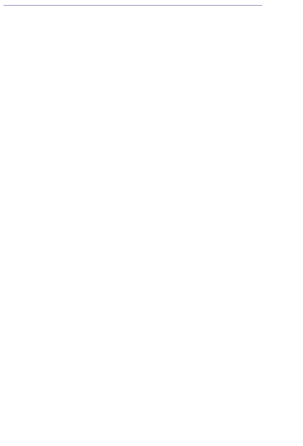
We shall show that the matrix

has only two independent components.

Consider the operators

acting on a matrix which are defined by

Here we again imply integration over internal frequencies and momenta. Using

the definition of the

operators and the normalization condition eqn (9.20) for

the regular functions we find

(9.26)

Consider the eigen-matrices of these operators

(9.27)

Each of these operators has four eigen-matrices belonging to four eigenvalues. It

is easy to check that the eigen-matrix

belonging to a nonzero eigenvalue

of the operator is simultaneously an eigen-matrix of the operator with

eigenvalue zero, and vice versa: the eigen-matrix

belonging to a nonzero

eigenvalue

of the operator is simultaneously an eigen-matrix of the

operator

with eigenvalue zero. To see this, we apply the operator to the

first equation (9.27) using eqn (9.26) and obtain

. We can also

apply

. to the second equation (9.27) to get . Applying the

operator

twice to the eigen-matrix we have

Applying the operator again we find . In the same way

we get

. Therefore, the four eigenvalues of the operator

are and twice degenerate . The

corresponding eigen-matrices

are simultaneously the eigen-

matrices of the operator

with the eigenvalues 0, 0, +2, and 2, respectively.

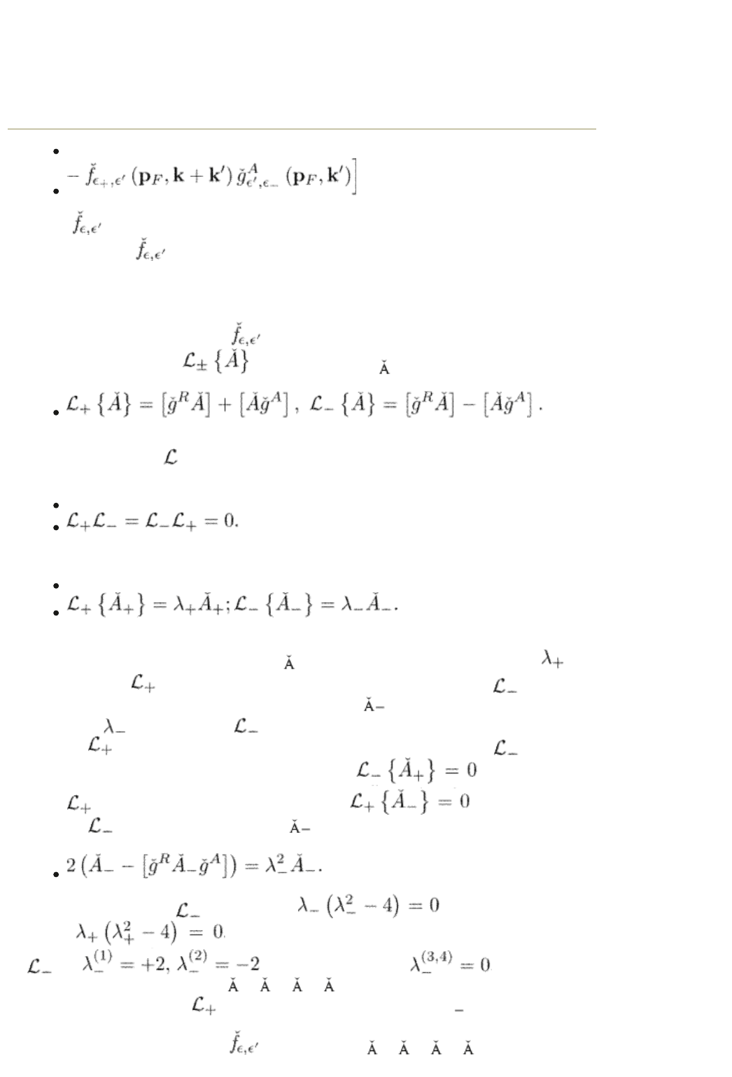
Let us now expand the matrix

in the matrices

We have

Kopnin, Nikolai, Senior Scientist, Low Temperature Laboratory, Helsinki University of

Technology, and L.D. Landau Institute for Theoretical Physics, Moscow

Theory of Nonequilibrium Superconductivity

Print ISBN 9780198507888, 2001

pp. [176]-[180]

Oxford Scholarship Online: Theory of Nonequilibrium Supe... http://www.oxfordscholarship.com/oso/private/content/phy...

第1页共6页 2010-8-8 15:51

It is clear that the coefficients and will not appear in the total Green

function

because the matrices

correspond to zero

eigenvalues of the operator

. Therefore, the matrix in eqn (9.25) has

only two

end p.176

independent components and . The two remaining coefficients

and can be chosen arbitrarily. For, example, one can choose them in such a

way as to make the function diagonal

(9.28)

This form of presentation for the distribution function was introduced by Schmid

and Schön (1975) and by Larkin and Ovchinnikov (1977) We note that, in

equilibrium,

where, as in eqn (8.9),

We use this form of presentation of the distribution function throughout the

book. Another choice for the free parameters

and has been suggested

by Shelankov (1985). It has an advantage in some cases when the relation to

the Boltzmann kinetic equation is considered.

In Chapter 10 we discuss the generalized two-component distribution function in

detail and derive the kinetic equations which determine f

(1)

and f

(2)

. The obtained

solutions will be used for various applications later in this book. In the rest of the

present chapter, we consider several examples of a direct implementation of the

Eliashberg equations in their original form.

9.3 S-wave superconductors with a short mean free path

Here we discuss an approach which can be used for superconductors with an

impurity mean free path

. This limit is realized for some s-wave

superconducting alloys. For d-wave superconductors, where always

this approach can also be used in a close vicinity of the critical temperature such

that

(T) already exceeds . We consider the d-wave case later in Section 11.3

while concentrating here on s-wave superconductors. The method is similar to

the one used in Section 5.6 to derive the Usadel equations.

The gradients of the order parameter and of other physical quantities are

generally of the order of

(T) and are thus small compared with . We can

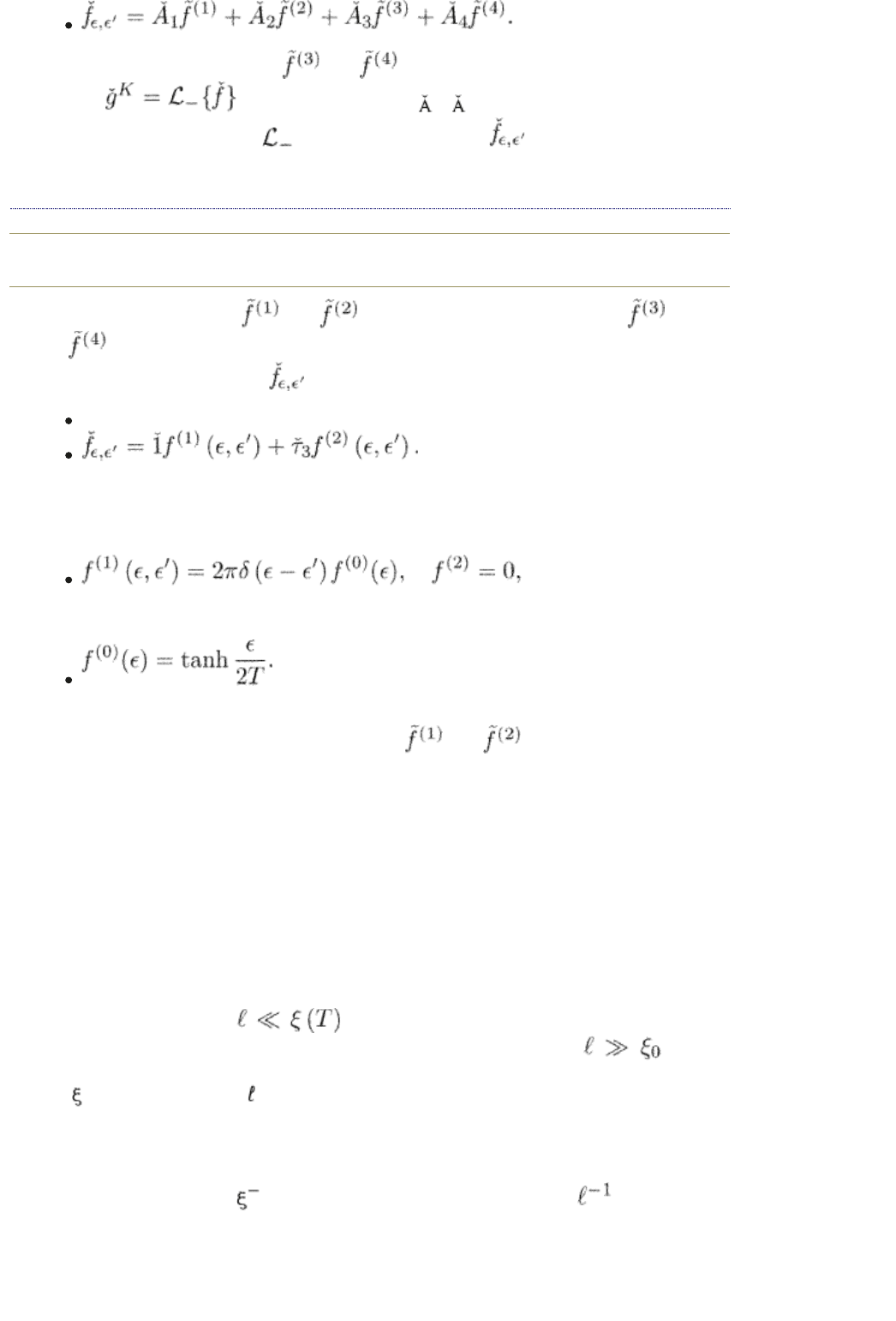
use a “hydrodynamic” approximation, assuming that the Green functions are, to

the first approximation, independent of the momentum direction, and restrict

ourselves to the first correction in small gradients. Since these corrections are

vectors, we write

PRINTED FROM OXFORD SCHOLARSHIP ONLINE (www.oxfordscholarship.com)

Oxford Scholarship Online: Theory of Nonequilibrium Supe... http://www.oxfordscholarship.com/oso/private/content/phy...

第2页共6页 2010-8-8 15:51

for all (retarded, advanced, and Keldysh) Green functions. Here is the unit

vector in the momentum direction, and

denotes an average over the

momentum directions in accordance with eqns (5.72) or (5.73). Both

and

are independent of the momentum direction. The vector part of the Green

function is small compared to its averaged value

end p.177

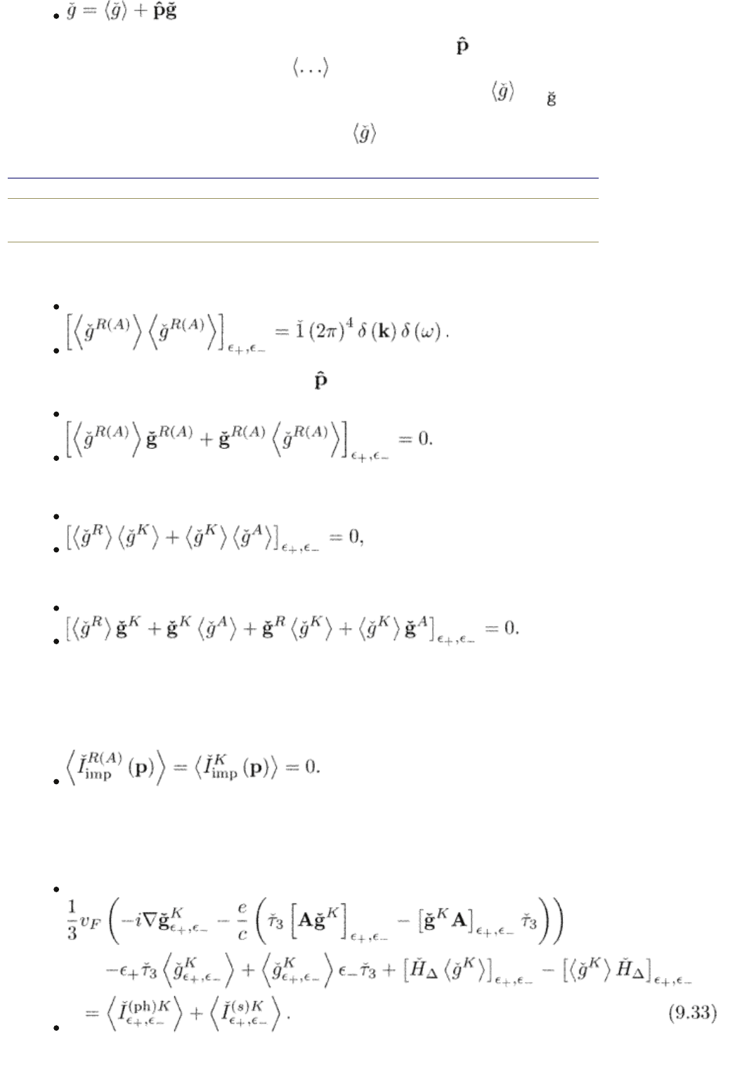
Averaging of the normalization condition eqn (9.20) gives for the regular

functions

(9.29)

Averaging it with the momentum direction results in

(9.30)

For the Keldysh function we have from eqn (9.24)

(9.31)

and

(9.32)

The impurity collision integrals for nonmagnetic scattering eqn (9.14) or (9.16)

are expressed through nonmagnetic self-energies defined by eqn (5.76). The

nonmagnetic collision integrals vanish after averaging over the momentum

directions:

Using this fact, we can simplify the quasiclassical equations in the same way as it

has been done in Section 5.6. On the first stage, we average the kinetic equation

over directions of the momentum. For the Keldysh function we get from eqn

(9.2) in coordinate representation

(9.33)

Here

PRINTED FROM OXFORD SCHOLARSHIP ONLINE (www.oxfordscholarship.com)

Oxford Scholarship Online: Theory of Nonequilibrium Supe... http://www.oxfordscholarship.com/oso/private/content/phy...

第3页共6页 2010-8-8 15:51

We note here an import ant difference between s-wave and d-wave

superconductors. For the s-wave case, the average of

does not disappear

because

is independent of the momentum directions. On the contrary, for a

d-wave case, this average vanishes.

Since the largest part of the total collision integral associated with lion magnetic

impurities disappears after averaging we have to keep other terms. In the

phonon and spin-flip collision integrals, one can replace the full Green

end p.178

functions by their averaged parts using smallness of the vector parts. We have,

for example

(9.34)

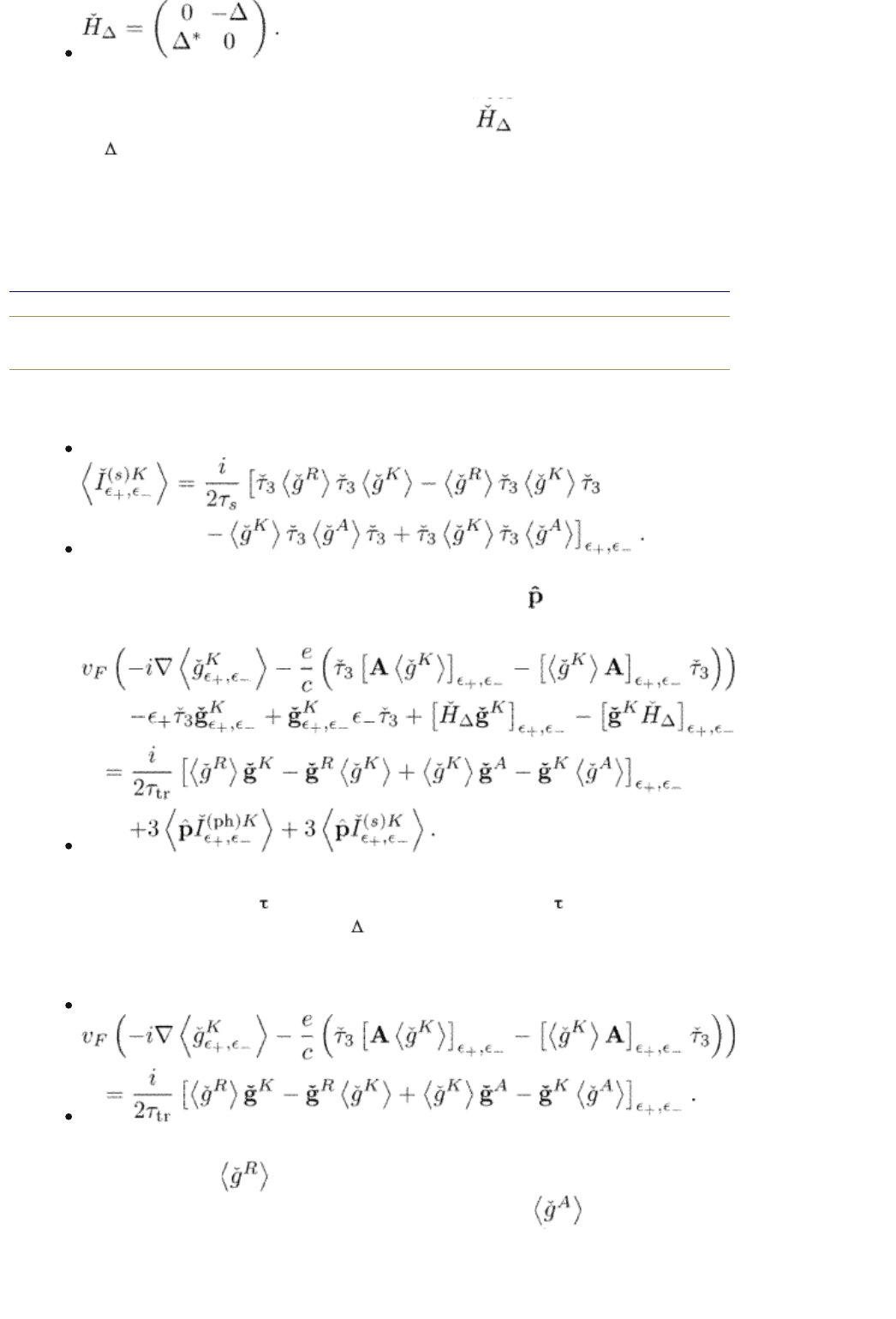
Let us now multiply eqn (9.2) by the momentum unit vector and average over

its directions. We obtain

We use eqn (5.80) here and the definition eqn (5.81) of the transport mean free

time. The relaxation rate 1/

is usually large compared with 1/

. In the dirty

limit it is also large compared to T and

, to say nothing about the electron-

phonon relaxation rate. Therefore, we can neglect the corresponding terms here

and obtain

(9.35)

This equation allows one to find the vector part of the Keldysh function. Let us

multiply eqn (9.35) by

from the left and integrate over internal

frequencies and momenta, then multiply eqn (9.35) again by

from the

right and subtract the two equations. Using eqns (9.29)–(9.32) we obtain

PRINTED FROM OXFORD SCHOLARSHIP ONLINE (www.oxfordscholarship.com)

Oxford Scholarship Online: Theory of Nonequilibrium Supe... http://www.oxfordscholarship.com/oso/private/content/phy...

第4页共6页 2010-8-8 15:51

The r.h.s. can also be written as

Having found the vector part from this equation, we can then use it to determine

the averaged functions from eqn (9.33). However, further transformations of

these

end p.179

equations cannot easily be performed in a general case. We shall consider some

examples later.

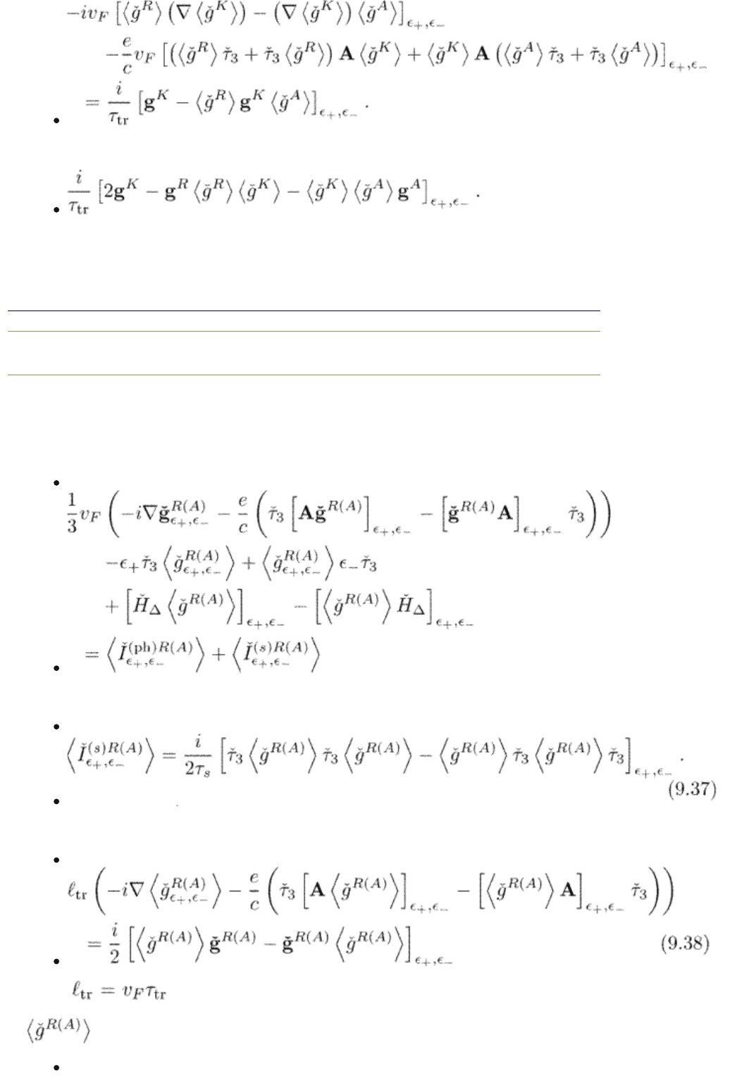
The equations for regular functions can be obtained in the same way. The

averaged equation is

(9.36)

where

(9.37)

The vector part is

(9.38)

where . The vector part of the regular functions can he found

using the normalization of eqns (9.29)–(9.30). Multiplying eqn (9.38) by

from the left, we get

(9.39)

PRINTED FROM OXFORD SCHOLARSHIP ONLINE (www.oxfordscholarship.com)

Oxford Scholarship Online: Theory of Nonequilibrium Supe... http://www.oxfordscholarship.com/oso/private/content/phy...

第5页共6页 2010-8-8 15:51