Hooke R.L. Principles of glacier mechanics

Подождите немного. Документ загружается.

Temperature distributions far from a divide 131

Table 6.2. Values of parameters in Equation (6.34)for

Site 2 in Greenland and Byrd Station in Antarctica

Site 2 Byrd Station

α −0.004 27 −0.001 61

,ma

−1

17 15

λ,Km

−1

−0.011 −0.008

,ma

−1

0.4 0.2

∂θ/∂z,Km

−1

0.001 15 0.000 24

(ε˙

H + b

),ma

−1

0.031 −0.018

Note that ∂θ/∂z is measured below 150 m depth.

only a short time interval. However, suppose we can measure u, α, λ, b

and ∂θ/∂z and have reason to believe that ∂θ

/∂t is negligible. Then,

Equations (6.34)or(6.35) can be solved for (ε˙

H + b

). Two examples

are shown in Table 6.2. The results, a 0.031 m a

−1

thickening rate at

Site 2 in Greenland and a 0.018 m a

−1

thinning rate at Byrd Station in

Antarctica, are surprisingly reasonable.

While potentially providing a sensitive measure of the state of health

of an ice sheet, this technique is probably not especially useful because

moderately deep boreholes are needed to obtain ∂θ/∂z, and ∂θ

/∂t is

not known well enough. However, the derivation of Equations (6.34) and

(6.35) serves to emphasize that, in general, as one moves away from the

divide, temperature gradients near the surface of an ice sheet become

positive; that is, the temperature decreases with depth (decreasing z). We

now turn our attention to a more sophisticated model that enables us to

investigate such temperature distributions deep in the ice and far from a

divide.

Temperature distributions far from a divide

The Column model

Budd et al.(1971) solved Equation (6.13)inamore general form than

those we have considered so far. Calculations using their model, which

they refer to as the Column model, can be done by hand.

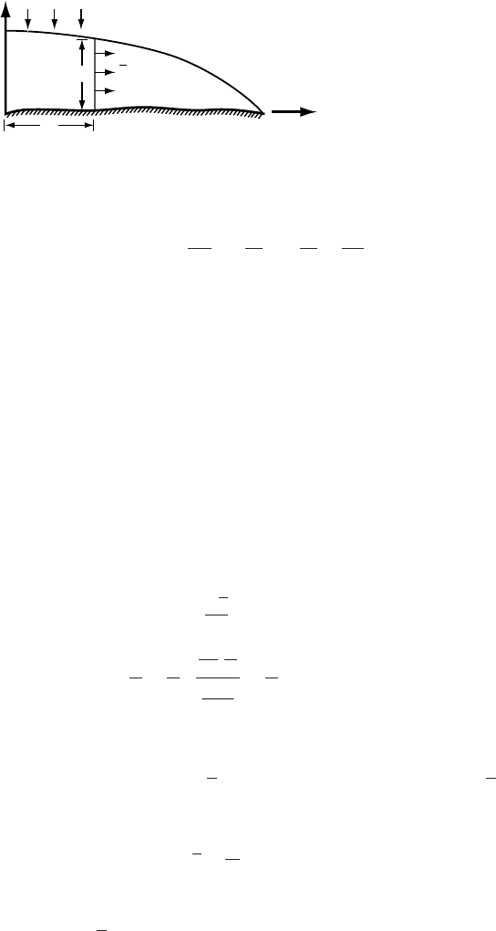
The coordinate system they use is shown in Figure 6.10. The tem-

perature proﬁle is to be calculated at a point a distance χ from the

divide. Starting again with Equation (6.13), we restrict the model to two

dimensions, thus eliminating derivatives in the y-direction; we assume

that temperature gradients in the x-direction are sufﬁciently small that

132 Temperature distribution in polar ice sheets

(x)

Figure 6.10. Coordinate

system and parameters

involved in Column model

calculations.

their derivative is negligible; and we assume a steady state. With these

assumptions, Equation (6.13) becomes:

0 = κ

∂

∂z

− u

∂θ

∂x

− w

∂θ

∂z

ρC

(6.36)

Let us now consider the strain heating term, Q/ρC.From Equation (6.9)

it will be seen that this term increases approximately as d

,where d is the

depth below the surface. In other words, because the strain rate increases

rapidly near the bed, most of the strain heating occurs in the basal few

meters of ice. (The student may ﬁnd it interesting to study this effect

by solving Equation (6.13) with the assumption that all advection terms

and the horizontal conduction terms are negligible, and that a steady

state exists. Equation (6.9)isused for Q/ρC. The problem is most easily

tackled by using a coordinate system in which the z-axis points vertically

downward.) Recognizing that signiﬁcant strain heating occurs only near

the bed, Budd (1969) assumed that it occurs only at the bed, and that

this heat could thus be added to the geothermal ﬂux. The basal boundary

condition, β

, thus becomes:

= β

(6.37)

maK

1Nm = 1J

and Q/ρC is set to zero. Here, as before, β

is the gradient required to

conduct the geothermal ﬂux upward into the ice; τ

is the basal drag,

approximated by ρgdα; and

u is the mean horizontal velocity. For u at

χ we use the balance velocity:

u =



(x ) dx (6.38)

(Equation (5.1)). In calculations, care must be taken to ensure that the

sign of the (τ

u)/K term is the same as that of β

; this sign is determined

by the choice of coordinate axes.

Temperature distributions far from a divide 133

We turn now to the term u · ∂θ/∂x in Equation (6.36). In Equation

(6.34)weset ∂θ/∂x = αλ,asthis is the rate at which the atmospheric

temperature increases as one moves to lower elevations along the ice

surface. This is, therefore, the rate at which near-surface ice must warm as

a result of horizontal advection. If the glacier surface slope is sufﬁciently

low, the deeper ice will warm at the same rate, with negligible lag. This

led Budd (1969)tosuggest that, to a reasonable ﬁrst approximation,

u ·∂θ/∂x can be replaced with uαλ in Equation (6.36). The consequences

of this assumption are discussed below.

With the additional substitution of (w

− w

)z/H for w, Equation

(6.36) becomes:

− (w

− w

)

dθ

= uαλ (6.39)

which is to be solved by using the boundary condition of Equation (6.37).

Here, w

and w

are the vertical velocities at the surface and bed respec-

tively; w

can be calculated from the submergence velocity (Equation

(5.26)) when b

, u

, and α are known. If the velocity at the bed is assumed

to be parallel to the bed, w

can be estimated from knowledge of u

and the

bed slope. Assuming that u

= u = u

is probably a reasonable approx-

imation in this calculation, but knowing

u, one could also calculate u

and u

from Equations (5.18) and (5.19).

The solution to Equation (6.39)is(Budd, 1969; Budd et al., 1971):

θ(h) = θ

−

[

erf (ζ H ) − erf (ζ h)

]

−

uαλH

− w

)

[

E(ζ H) − E(ζ h)

]

(6.40)

where:

erf (x ) =



−t

E(x) =







−y







ζ =



− w

2H κ



1/2

Note that this solution uses Budd’s deﬁnition of the error function, erf (x).

E(x)isthe integral of a function known as Dawson’s integral (the quantity

in square brackets), and it too has been tabulated. A plot of it for a

reasonable range of ζ is shown in Figure 6.5.

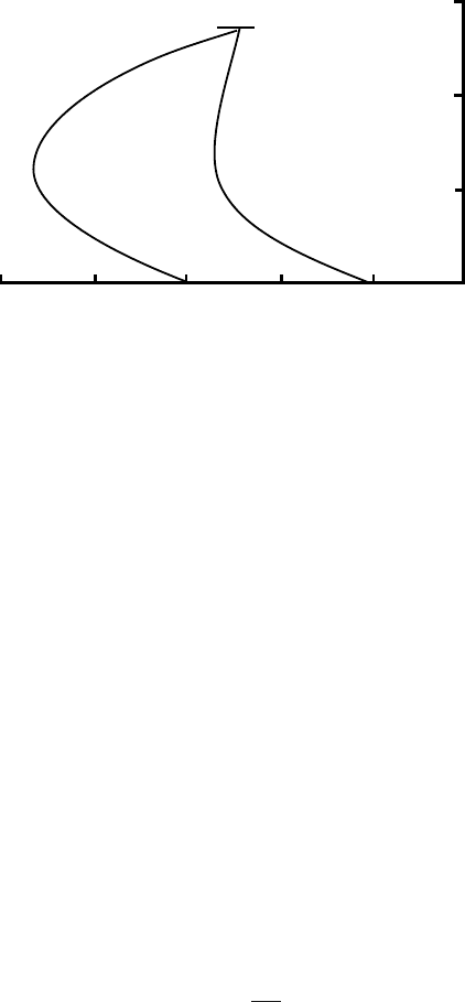
Temperature proﬁles can be calculated readily by using Equation

(6.40) and Figure 6.5.Atypical one is shown in Figure 6.11 (proﬁle (a)).

134 Temperature distribution in polar ice sheets

−50 −40 −30 −20 −10 0

Temperature,

1500

1000

500

Height above bed, m

Glacier surface

(b) (a)

Figure 6.11. Temperature

proﬁles calculated from

(a) Equation (6.40) and

(b) Equation (6.41). The

following values of the

parameters, approximately

appropriate for Camp

Century, Greenland, were

used in the calculations:

α =−0.01, u = 15ma

−1

λ =−0.01 K m

−1

κ = 37.2 m

−1

, H = 1368 m,

=−24

◦

C, and

=−0.0508 K m

−1

The minimum temperature occurs at some depth below the glacier sur-

face. This represents, as in Figure 6.9, cold ice that is advected downward

and laterally from some point further upglacier where the surface is at

a higher elevation and hence colder. However, the Column model does

not include this longitudinal advection rigorously, but simply speciﬁes

awarming rate. Thus the temperature at depth is only an approximation

that becomes better as the warming rate decreases. This approximation

is best, therefore, where surface slopes (α) and lapse rates (λ) are lowest.

Both the magnitude and the curvature of the positive temperature gra-

dient near the surface are adjusted so that heat conducted downward from

the surface, in combination with heat advected downward, is sufﬁcient to

warm the ice everywhere above the point of minimum temperature at the

rate uαλ. Ice below this point is warmed at this rate by heat from the bed –

both geothermal and frictional. When the warming rate at depth that is

speciﬁed (by representing it by uαλ)islarger than that in the natural

situation being modeled, the positive temperature gradient at the surface

becomes too high, and the temperatures at depth, thus, too cold.

Further insight into the mathematical properties of the solution can

be gained by comparing the proﬁle calculated from Equation (6.40) with

one calculated from:

∂

∂x

= uαλ (6.41)

together, again, with the boundary condition of Equation (6.37). (The

integration of Equation (6.41)isleft as an exercise for the reader.) This

is proﬁle (b) in Figure 6.11. Equations (6.39) and (6.41) differ in that the

vertical advection term is omitted in Equation (6.41). By analogy with

our discussion of Equation (6.24) and Figure 6.7, one might think that

Englacial and basal temperatures 135

because vertical advection moves cold ice downward from the surface,

omission of this term would make proﬁle (b) warmer than proﬁle (a) at

depth. However, in this case the ice at depth is colder than that at the

surface, and because the vertical advection term operates on ice at the

surface at the point where the proﬁle is being calculated, not at some

point upglacier therefrom, the ice advected downward is warmer than

the ice at depth. As a result of this downward advection of heat, included

in Equation (6.40), the uαλ warming rate does not need to be satisﬁed

entirely by conduction from the surface in proﬁle (a).

Englacial and basal temperatures along a ﬂowline

calculated using the Column model

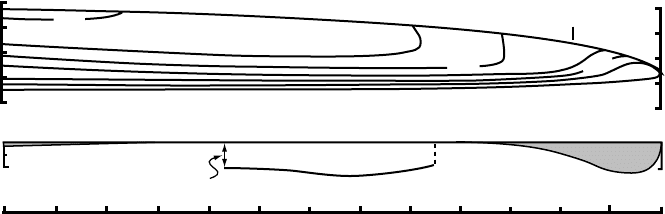
Let us now consider the temperature distribution along a ﬂowline cal-

culated with the use of the Column model (Figure 6.12). The original

objective of the modeling shown in Figure 6.12 wastoinvestigate the

possibility that, along the margin of the Laurentide Ice Sheet in North

Dakota, there could have been a ∼2 km-wide zone in which the ice was

frozen to the bed. Such a temperature distribution is implied by glacial

landforms, as discussed further below (Moran et al., 1980). Thus, the

ﬂowline modeled was assumed to extend from Hudson Bay to North

Dakota.

In the model, the accumulation rate was assumed to be 0.20 m a

−1

65 km upglacier from the equilibrium line, and to decrease linearly to

0.05 m a

−1

at the divide, and to 0 at the equilibrium line. The decrease

in b

toward the divide is consistent with the present accumulation pat-

tern in Antarctica (Figure 3.9) and northern Greenland, although not

southern Greenland (Zwally and Giovinetto, 2000). In the ablation area,

the ablation rate increased linearly downglacier from the equilibrium

line, and the rate of increase was adjusted to provide a balanced mass

budget. The horizontal velocity was approximated by the balance veloc-

ity (Equation (5.1) modiﬁed to allow for divergence of the ﬂowlines).

The ice sheet proﬁle was adjusted to provide the shear stress necessary

to yield this horizontal velocity, using a relation similar to the ﬁrst of

Equations (5.19) with a sliding law to estimate u

. Isostatic depression

of the earth’s crust was included. The vertical velocity was calculated

from the submergence or emergence velocity relation (Equation (5.26)),

and was assumed to decrease linearly with depth (Equation 6.15). The

temperature at the margin was −7.5

◦

C. The temperature along the sur-

face was calculated assuming a lapse rate of −0.01 K m

−1

, and making

an empirical correction for warming effects of percolating melt water.

The geothermal ﬂuxes used were appropriate to the geologic terrane

136 Temperature distribution in polar ice sheets

along the ﬂowline. To circumvent certain problems, discussed later, it

was assumed that the warming rate was

uαλ instead of uαλ.

Several features of the temperature distribution in Figure 6.12 merit

comment.

The downward and outward advection of cold ice is represented by the

reversal in slope of the −20

◦

C and −25

◦

C isotherms ∼900 km from

the divide.

The progressive compression of the isotherms near the bed

downglacier from the divide reﬂects the outward increase in basal

temperature gradient as strain heating increases.

Basal melting occurs over the ﬁrst 250 km of the ﬂowline because the

accumulation rate here is low, and downward advection of cold ice

is, thus, less important than it is further downglacier. A more realistic

vertical velocity distribution would lead to more melting here, while

a higher accumulation rate would lead to less melting.

Between ∼250 and ∼420 km from the divide, half of the meltwater

formed in the ﬁrst 250 km is refrozen to the base. This keeps the bed at

the pressure melting temperature. The rest of the water was assumed

to have drained away into the bedrock. (Had it been assumed, instead,

that more of the meltwater stayed at the ice/bed interface, the zone of

subfreezing temperatures between ∼420 and ∼840 km from the divide

would be smaller or absent.)

The zone of subfreezing basal temperatures between ∼420 and

∼840 km owes its existence to increased downward advection of cold

ice as the accumulation rate increases outward.

Basal melting resumes downglacier from ∼840 km as strain heating

warms the basal ice. It becomes particularly important in the ablation

area where upward vertical velocities decrease the basal temperature

gradient, thus trapping more heat at the bed.

The basal frozen zone at the margin, barely visible at the scale of the

ﬁgure, is a result of cold atmospheric temperatures at the margin and

decreasing vertical velocity as the margin is approached. The verti-

cal velocity decreases because, as the surface slope steepens, a greater

fraction of the ablation rate is balanced by the u

tan α term in the emer-

gence velocity. In addition, it is assumed that the meltwater formed in

the outer ∼500 km of the glacier leaves the system as groundwater or

by wayoflocalized subglacial conduits.

Even though the Column model is relatively crude in comparison

with numerical models being used today, it does reproduce what are

probably the essential features of the temperature distribution at the base

of a continental-scale ice sheet with an ablation zone of signiﬁcant width,

Englacial and basal temperatures 137

Distance from divide, km

0 500 1000 1300

−2

Basal melt rate

Pressure

melting

Basal temperature

mm a

−1

Basal melt rate

-30

-20

-10

Eq. line

−1

Elevation a.s.l, km

Figure 6.12. Temperature distribution along a ﬂowline calculated with the use

of the Column model. The bed is at the pressure melting temperature except in

the section labeled “Basal temperature”. (From Moran et al., 1980, Figure 6.

Reproduced with permission of the International Glaciological Society.)

namely: (1) melting beneath the divide if the accumulation rate is suf-

ﬁciently low and freezing otherwise; (2) in the former case, a zone of

freeze-on in the lower part of the accumulation area followed by a pos-

sible zone in which the ice is frozen to the bed; (3) melting beneath the

ablation area; and (4) a possible frozen toe in areas where marginal tem-

peratures were relatively cold. The distribution of these zones depends

on b

, β

, and θ

.Temporal changes in b

and θ

due to climate change

will alter the basal temperature distribution, but there will be a lag

of order 10

years between any change in climate and a response at

the bed.

The fact that water from melting basal ice ﬂows downglacier along

the bed and refreezes is consistent with observations of layers of dirty

ice, several meters thick, that were encountered at the bottoms of both the

Byrd Station, Antarctica, and the Camp Century, Greenland, ice cores.

In both cases, the dirt was dispersed throughout the ice, and the dirty

ice had fewer air bubbles than the overlying clean ice. In the Camp

Century core, the oxygen isotope ratios indicated that the basal dirty ice

was formed from water that originally condensed at lower temperatures

than the overlying ice. All of these observations are consistent with

melting of ice that originally formed at a higher altitude than the overlying

ice, downglacier ﬂow of that water along the bed, and refreezing of

the water incorporating dispersed dirt in the process. It is difﬁcult to

account for meters-thick layers of basal ice with dispersed dirt in any

other way, although regelation of ice downward into till is a possible

wayofentraining layers of dirt with higher debris content (Iverson,

1993).

138 Temperature distribution in polar ice sheets

A problem with high uαλ warming rates in the

Column model

As the warming rate required by the uαλ term in the Column model

increases, the curvature of the temperature proﬁle increases, and the

minimum and basal temperatures decrease (see Figure 6.11 and discus-

sion on p. 134). Near the equilibrium line, the downglacier warming rate

is high because meltwater percolating into the ﬁrn raises near-surface

temperatures. (In the modeling for Figure 6.12 this effect was included

by using an effective value of λ that is higher than the atmospheric lapse

rate.) If the ice at depth is assumed to be warming at the same rate, cal-

culated minimum temperatures in proﬁles near the equilibrium line are

often lower than the minima in proﬁles just upglacier. In plots such as

Figure 6.12, this appears as a pocket of cold ice beneath the equilibrium

line that is surrounded by warmer ice (Hooke, 1977,Figure 4c). Such a

temperature distribution is physically impossible; to have cooled off, this

ice would have had to have lost heat to colder ice, yet it is surrounded

by warmer ice.

To circumvent this problem, as noted, a warming rate of

uαλ was

used.

Basal temperatures in Antarctica – comparison

of solutions using the Column model and a

numerical model

The reliability and weaknesses of the Column model can be illustrated

further by comparing basal temperatures in Antarctica calculated using it

(Budd et al., 1971) with those calculated using a state-of-the-art numer-

ical model (Huybrechts, 1990). First, however, it is instructive to discuss

some general characteristics of the Antarctic ice sheet that affect the

temperature distribution.

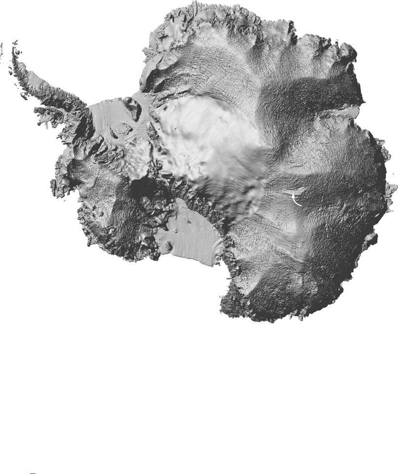
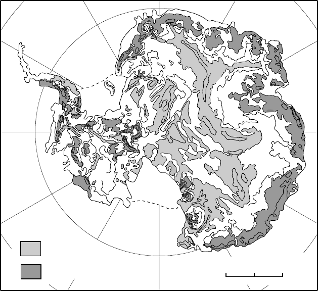
A digital elevation model (DEM) of the ice sheet is shown in

Figure 6.13 (Liu et al., 1999). By constructing this image with consid-

erable vertical exaggeration, Liu et al.have emphasized intricate details

of the surface topography, many of which would be difﬁcult to discern

were one standing on the surface of the ice sheet. Noteworthy is the

apparent roughness of parts of the surface. This is caused by undula-

tions with wavelengths of 4–10 km and amplitudes of only 5–10 m that

result from ﬂow over topography on the bed. Also of interest is the

remarkably ﬂat area labeled “Lake Vostok”. As discussed previously

(p. 99), this area is over a subglacial lake. Lake Vostok is the largest

of many subglacial lakes that have been detected through radio-echo

sounding.

Basal temperatures in Antarctica 139

Lake Vostok

Figure 6.13. Digital elevation model of Antarctica. From Liu et al., 1999.

(Courtesy of G. Hamilton.)

The basal drag in Antarctica, calculated from the surface proﬁle

and ice thicknesses, is shown in Figure 6.14.Incontrast to the situation

on valley glaciers, where τ

is typically between 0.05 and 0.15 MPa

(p. 85), the basal drag is below 0.05 MPa over most of Antarctica. Note

also that τ

decreases inland. The low accumulation rates near the center

of the ice sheet result in low balance velocities. Thus, the driving stresses

required to provide those balance velocities are also low. Because both

and u (Figure 5.2) increase toward the coast, the basal temperature

gradient, β

, also increases (Equation (6.37)). The geothermal gradient,

,isestimated to be only about 0.02 K m

−1

in East Antarctica, whereas,

owing to strain heating, β

is nearly ﬁve times that near the coast.

Basal temperatures calculated with the use of the Column model

and by Huybrechts (1990) are shown in Figures 6.15a and 6.15b,

140 Temperature distribution in polar ice sheets

Ice

shelf

Ice

shelf

≤ 40 kPa

≥ 80 kPa

1000 km

Figure 6.14. Basal drag in Antarctica calculated by Ph. Huybrechts, especially

for this book, using the model described in Huybrechts (2002).

respectively. In both maps one of the coldest spots is in central East

Antarctica, over a mountain range where the ice is only 1.5–2 km thick.

In nearby areas it is over 4 km thick. Both also predict basal melting

in the same areas in West Antarctica. However, there are important

systematic differences between the maps. Most obvious is the large

area of basal melting in East Antarctica in Huybrecht’s map. This is, in

part, attributable to the fact that Huybrechts used a geothermal ﬂux of

54 mW m

−2

,while Budd et al. used 50 mW m

−2

. This, however, cannot

account for so large a difference. Possible explanations for the remaining

difference are the use of an unrealistic linear decrease in w with depth in

the Column model and requiring that the warming rate at depth equal that

at the surface. As we have seen, the former can lead to basal temperatures

that are too cold (Figure 6.6), and the latter can result in temperature

gradients at the surface that are too high (Figure 6.11), thus also making

deeper temperatures too cold. In contrast, Huybrecht’s model predicts

colder temperatures in Queen Maud Land. This appears to be because