Hooke R.L. Principles of glacier mechanics

Подождите немного. Документ загружается.

Submergence and emergence velocities 91

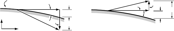
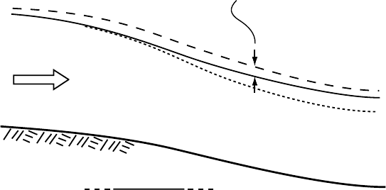
Ice surface

tan a

(a) (b)

tan a

Figure 5.10. Diagrams illustrating (a) submergence, and (b) emergence

velocities.

Submergence and emergence velocities

Earlier (Equation (5.1)), we gained insight into the magnitude of the

horizontal velocity by considering a glacier in a steady state, such that

its surface proﬁle remained unchanged. Let us now use this idealization

to study vertical velocities. In such a steady state, the surface in the

accumulation area must everywhere be sinking at a rate that balances

accumulation, and conversely in the ablation area. Thus, the vertical

velocity at the surface, w

,isclearly related to the net balance rate, b

Remembering that a point on the surface is also moving with a horizontal

velocity, u

, and that the surface has a slope, α,weﬁnd that the appropriate

relation is (Figure 5.10):

=−w

+ u

tan α (5.26)

Here, we have taken the x-axis as horizontal and positive in the

downglacier direction, and the z-axis as positive upward. Thus, in the

accumulation area, both w

and α are negative and, owing to the rela-

tive magnitude of the two terms on the right-hand side of the equation

(see Figure 5.10a), the minus sign in the equation makes the right-hand

side positive. In the accumulation area, the right-hand side is called the

submergence velocity.

Equation (5.26) also applies in the ablation area (Figure 5.10b),

except that here w

is positive so both terms on the right-hand side

take on negative values. Thus b

is negative, reﬂecting ablation. Here,

the right-hand side is called the emergence velocity.

Clearly, the submergence and emergence velocities are deﬁned for

any point on a glacier surface. However, they equal b

only in the ide-

alized steady-state situation that we have speciﬁed. This is because b

varies from year to year, and because, even averaged over several years,

glaciers are rarely in a steady state. Put differently, if the accumulation

rate consistently exceeds the submergence velocity and the ablation rate

92 The velocity ﬁeld in a glacier

consistently falls short of the emergence velocity, the glacier is becoming

thicker and will advance, and conversely.

Other possibilities can also be visualized. For example, if the equality

in Equation (5.26) holds everywhere except in the lower part of the

ablation area where the ablation rate exceeds the emergence velocity, the

glacier may be in the ﬁnal stages of adjustment to a climatic warming.

The implication of such a situation would be that the accumulation area

has essentially adjusted to the warming, but the glacier is still retreating

slightly.

We have shown that on a glacier that is in a steady state and that

has a balanced mass budget, the velocity ﬁeld at the surface is related to

.Itisinstructive to consider in greater detail the physical mechanisms

behind this relation. In this case, b

is the independent variable, and

the velocity ﬁeld is the dependent variable. (In a larger system involv-

ing glacier–climate interactions, b

would be dependent upon the cli-

mate.) The physical mechanism by which b

and the velocity ﬁeld are

related is viscous ﬂow, in which the ﬂow rate increases with the driving

stress, ρghα. If the velocities are, say, too low (in absolute value), the

submergence velocity will be less than the accumulation rate so the

glacier will become thicker in the accumulation area (Figure 5.10a).

Similarly, the emergence velocity will be less than the ablation rate, so

the glacier will become thinner in the ablation area (Figure 5.10b). The

slope of the glacier surface thus increases. The increase in slope, cou-

pled with the increase in thickness in the accumulation area, increases

the driving stress and hence u

. Because u = 0atthe head of the glacier

and at the terminus, an increase in u

in the middle makes ∂u/∂x more

extending in the accumulation area and more compressive in the ablation

area. Thus, by the arguments leading to Equation (5.26), |w

| increases.

The increases in both u

and |w

| tend to restore the steady state.

Flow ﬁeld

We now have the tools needed to make a ﬁrst-order estimate of the ﬂow

ﬁeld in a glacier, given b

(x). In a steady-state situation, Equation (5.1)

gives the depth-averaged horizontal velocity, u(x), which is probably

sufﬁcient for most applications. However, various levels of sophistication

could be added; Equations (5.16) (with z =H) and (5.19) could be solved

simultaneously for u

and u

, and Equation (5.16) could then be used

to estimate the variation in u with depth. This would give u(x,z). Then,

Equations (5.24) and (5.26) provide a reasonable ﬁrst estimate of w(x,z).

Thus, one could plot vectors u and w at a large number of points in a

glacier cross section and sketch ﬂowlines based on these vectors. The

result would be ﬂowlines much like those in Figure 3.1.

Flow ﬁeld 93

It may be worthwhile studying Figure 3.1 in connection with the

above equations to develop an intuitive sense of why the ﬂowlines appear

as they do. From Equation (5.26) and Figure 5.10,itisclear that the ver-

tical velocity must be downward in the accumulation area and upward in

the ablation area. Owing to the slope of the glacier surface, the location

where w

= 0isnot at, but rather slightly downglacier from, the equi-

librium line (Equation (5.26)). From Equation (5.1)itisobvious that u

increases outward from the divide, reaching a maximum again not at,

but rather slightly downglacier from, the equilibrium line. Because the

variation in w

is small compared with that in u

, the resultant velocity

vectors plunge most steeply near the divide and ascend most steeply near

the margin, as u

is low in these locations. In fact, at the divide on a polar

ice sheet, u

= 0sothe vector points directly downward. Near the bed,

is low so the vectors approach parallelism with the bed.

In summary, ﬂowlines tend to be downward in the accumulation area

and upward in the ablation area. At the bed they are parallel to the bed

and at the equilibrium line (of our idealized steady-state glacier) they are

parallel to the surface. The ﬂowline starting at the divide on an ice sheet

will go straight downward until it reaches the bed, and then will follow

the bed, remaining strictly parallel to the bed in the absence of melting

or refreezing, until it emerges at the margin.

In the steady state, the volume of ice moving between two adjacent

ﬂowlines remains constant along the full length of these two ﬂowlines.

This is true by deﬁnition; material cannot cross a ﬂowline, so all material

that starts between two ﬂowlines must remain between them. A conse-

quence of this is that the velocity will be highest where the ﬂowlines are

closest together, as the ice is assumed to be incompressible. Thus the

highest velocities will be near the equilibrium line, as is evident from

Equation (5.1).

Steady-state conditions are, of course, a theoretical abstraction,

rarely if ever actually realized in nature. The annually averaged velocity

ﬁeld of a retreating or advancing glacier should not, however, differ too

signiﬁcantly from that described above. On the other hand, seasonal and

spatial variations in the velocity ﬁeld, particularly on valley glaciers, can

be appreciable. A number of studies have shown that when water from

the surface is able to reach the glacier bed, glaciers speed up in the sum-

mer (see Figure 12.10). This is because water pressures increase, thus

increasing the sliding speed. There are even diurnal variations in surface

speed (see Figures 7.8 and 7.23). Because sliding speeds are highest

beneath the centerline of the glacier (Figure 5.8), seasonal accelerations

are highest here. These accelerations result in measurable changes in the

magnitude and direction of velocity vectors, both at the surface and at

depth (Hooke et al., 1992). In contrast, Harper et al. (2001), in a study

94 The velocity ﬁeld in a glacier

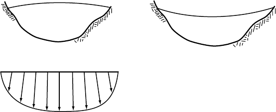
(a) (b)

(c)

Figure 5.11. Schematic cross

sections of a valley glacier in

(a) the ablation area, and (b)

the accumulation area; and

showing the transverse

variation in u

in the ablation

area.

utilizing 31 boreholes in the central part of Worthington Glacier, Alaska,

did not ﬁnd seasonal variations. They did, however, ﬁnd signiﬁcant spa-

tial variations at a length scale of tens of meters. In a transverse cross

section of the glacier, there were variations in horizontal speed of as

much as 5% that did not seem to be related to side drag, but may have

been caused by longitudinal stresses originating in an ice fall higher on

the glacier.

Transverse proﬁles of surface elevation on a

valley glacier

In the ablation area of a valley glacier, transverse proﬁles of surface

elevation are commonly convex upward (Figure 5.11a), whereas in the

accumulation area they are concave upward (Figure 5.11b). This can be

understood by considering the emergence and submergence velocities.

In a steady-state situation, w

cannot be zero along the margins of a

glacier in either the accumulation area or the ablation area because there

is accumulation or ablation, respectively, in these locations. However,

the ice thickness goes to zero at the margin. Thus to provide a downward

near the margin in the accumulation area, ice must be drawn away

from the valley sides, and conversely in the ablation area. The transverse

surface slopes, towards the center of the glacier in the accumulation area

and away from the center in the ablation area, provide the forcing for this

ﬂow.

Consideration of transverse variations in the emergence and submer-

gence velocities provides insight into lateral variations in w

and into the

mechanism of adjustment of transverse proﬁles. Let us start with the

ablation area. Horizontal velocities are normally highest near the center

of a glacier and decrease towards the margins owing to drag on the valley

sides (Figure 5.11c), in much the same way that velocities decrease with

depth owing to drag on the bed. The ablation rate, however, is normally

Transverse proﬁles of surface elevation 95

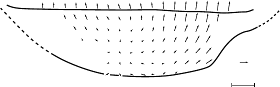
2 m a

−1

100 m

Figure 5.12. Transverse

velocity ﬁeld measured in a

cross section of Athabasca

Glacier by Raymond (1971,

Figure 12). (Reproduced with

permission of the author and

the International Glaciological

Society.)

approximately constant across the glacier. It may, in fact, be somewhat

higher near the margins as a result of heat radiated or advected from dark

rocks of the valley walls. The longitudinal surface slope, α, will also be

approximately constant across the glacier. Thus, from Equation (5.26)

or Figure 5.10b,itisclear that w

must be higher near the margins than

along the centerline, as illustrated in Figure 5.12.

The process by which the transverse proﬁle in the ablation area is

adjusted is easy to understand. Consider what would happen if the proﬁle

were ﬂat and w

were constant along this proﬁle. Suppose the ablation

rate equals the emergence velocity at the centerline. Along the margins

where u

is lower, b

would exceed the emergence velocity, so the glacier

surface would decrease in elevation, leading to the convexity that is com-

monly observed. The resulting transverse surface slope would force a

transverse component to the ﬂow. Because the valley walls inhibit such

ﬂow, a transverse compression develops, thus increasing the rate of ver-

tical extension near the sides of the glacier (assuming no compensating

change in the longitudinal strain rate). The magnitude of the transverse

slope would continue to increase, thus increasing w

, until the emergence

velocity equaled the ablation rate. Of potential interest in trying to under-

stand landforms produced by glacial erosion is the fact that the trans-

verse component of the ﬂow is apparently greatest near the bed, accord-

ing to measurements made by Raymond (1971)onAthabasca Glacier

(Figure 5.12).

In the accumulation area, the situation is reversed. As in the ablation

area, u

is lower near the margin, so if the longitudinal component of α is

approximately constant across the glacier, u

tan α will be less negative

near the margin than on the centerline. In addition, b

is likely to be higher

along the margin owing to drifting and avalanching. The ﬂow ﬁeld thus

has to develop in such a way that w

is more negative (downward) near

the margins than near the centerline (Equation (5.26)orFigure 5.10a).

However, the ice is thinner near the margin so the longitudinal stretching

rate is likely to be lower, thus contributing less to a negative w

. Some-

how, w

must become more negative. The concave cross-valley proﬁles

(Figure 5.11b) that are typical of accumulation areas accomplish this.

96 The velocity ﬁeld in a glacier

To visualize the physical processes involved in this adjustment, con-

sider again a hypothetical case in which the transverse proﬁle is initially

ﬂat, rather than concave upward. In this case, there would be no trans-

verse component to the surface slope, and hence little or no transverse

component to the ﬂow. Flowlines would be parallel to the glacier mar-

gin, and longitudinal strain rates along ﬂowlines near the margin would

be too low to provide the negative w

needed to balance the accumu-

lation. In other words, the left-hand side of Equation (5.26)would be

larger than the right-hand side, and the glacier would become thicker

in this area. This thickening along the margins would continue as long

as the imbalance persisted, thus establishing the characteristic concave-

upward transverse proﬁle. The transverse surface slope would result in

a transverse component of ﬂow toward the center of the glacier, and

because glaciers normally increase in thickness rapidly away from the

margins, stretching rates are high along ﬂowlines that diverge from the

margin. The resulting transverse stretching provides the more negative

required near the margins.

If transverse proﬁles are generally convex upward in the ablation

area and concave upward in the accumulation area, it is interesting to

consider exactly where the transition between the two types of proﬁle

should occur. Let us return to our idealized steady-state glacier with a

balanced mass budget. At the equilibrium line on this glacier, b

= 0,

so from Equation (5.26) w

tan α.Asα<0 and u

> 0, w

must still

be somewhat negative (downward), as mentioned previously. The place

where w

=0issomewhat downglacier from the equilibrium line, where

= u

tan α.Itisapproximately at this point that one might expect the

transition to occur. Leonard and Fountain (2003), in a study of 40 glaciers,

found that this indeed was the case. For reasons that are not obvious,

the difference in elevation between the transition and the equilibrium

line increased systematically with elevation of the equilibrium line. The

location of the transition relative to the equilibrium line depends on b

, and α,soitwill vary from glacier to glacier.

Radar stratigraphy

Prior to World War II, pilots ﬂying over Greenland and Antarctica found

that their radar altimeters were giving unreliable data. Upon investiga-

tion, it was discovered that the radar waves were passing through the ice

sheet and reﬂecting from the bed (Waite and Schmidt, 1961). Thus was

born the tool of radio echo-sounding of glaciers (Gogineni et al., 1998).

Initially, the primary objective was to determine the thickness of the ice,

as previously gravity measurements, seismic proﬁling, and drilling were

the only techniques available to glaciologists for this purpose. However,

Radar stratigraphy 97

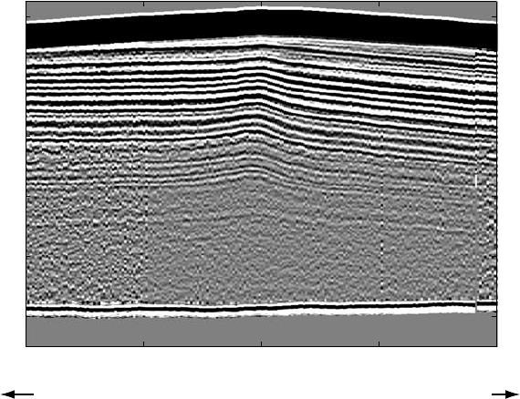
Surfa

Bed

10 5 0 5 10

−400

−200

200

400

600

Distance from summit, km

NorthSouth

Elevation above sea level, m

Figure 5.13. A20kmradar proﬁle across the divide of Siple Dome, Antarctica,

showing internal layering. The black band at the top is caused by interference

from radio waves passing directly through the air. (From Nereson et al., 1998,

Figure 2. Reproduced with permission of the International Glaciological Society.)

it was soon discovered that internal layering of glaciers and ice sheets

was also being imaged. By adjusting the frequency of the radio waves

and imposing sophisticated ﬁltering on the return signals, remarkably

sharp images of this layering are now being obtained routinely (Figure

5.13). Reﬂections are caused by subtle contrasts in the dielectric con-

stant. Those from shallower layers probably result from differences in

density; those from deeper layers are attributed to acidic fallout from

volcanic eruptions or to changes in impurity concentration associated

with climatic transitions (Morse et al., 1998). Accordingly, such lay-

ers are commonly assumed to be stratigraphic horizons, representing

isochrones, and they thus can be used to study the ﬂow ﬁeld and changes

in it over time.

A radar proﬁle (Figure 5.13) across the divide of Siple Dome, an

elongate high area in West Antarctica (see Figure 5.20), provides one

example of a feature that merited study. A bump is clearly visible

in the internal layering. The amplitude of this bump increases with

depth, reaching a maximum of ∼50 m. The bump suggests a change

in the vertical velocity outward from the divide. There are two possible

explanations for such a change (Nereson et al., 1998). As we discov-

ered above, ε˙

decreases with depth beneath a divide, so the deeper ice

98 The velocity ﬁeld in a glacier

is stiffer than that at the surface. Consequently, the vertical velocity

generally decreases more rapidly beneath the divide than it does on the

ﬂanks (Figure 5.9), so as layers form at the surface and are buried by

subsequent accumulation, they are draped over the stiffer plug. Because

this explanation is based on Raymond’s (1983) analysis of the vertical

velocity ﬁeld (Equations (5.24) and (5.25)), the resulting distortion of

the internal layering has become known as the Raymond bump. Alter-

natively, drifting or wind scouring may reduce the accumulation over

the divide, in which case the ﬂow ﬁeld would have to adjust so that w

waslower there. Thus, again, isochronous surfaces would be buried less

rapidly beneath the divide than on the ﬂanks.

Nereson et al. (1998) analyzed the layer shapes with the use of a

numerical ﬂow model. The modeling was complicated by the fact that

accumulation gradients are likely to exist across the divide even if drifting

has not resulted in a local low in b

. Unfortunately, the true accumulation

pattern is not known so these gradients had to be free parameters in the

modeling. In addition, the bump is offset to the north with increasing

height above the bed (Figure 5.13), suggesting migration of the divide.

The divide migration rate thus becomes another free parameter. With

this many free parameters it was possible to model the bump rather well,

but the relative contributions of a decrease in ε˙

and drifting could not be

evaluated. It seems likely that both are involved. The estimated migration

rate, based on the modeling, is ∼0.3 ± 0.2ma

−1

over the past several

thousand years.

In another example, Morse et al. (1998) found that beneath the divide

on Taylor Dome, Antarctica, shallower layers thickened southward while

deeper layers thickened northward. Isotopic and chemical variations in

a core were used to establish an age/depth time scale; it turned out that

the northward-thickening layers were deposited during the Late Glacial

Maximum (LGM). By using a numerical model of ice ﬂow, they also

found that the accumulation rate was much lower during the LGM. The

change in thickness gradient in the radar layering was then attributed to

a change in storm tracks during the LGM, with storms coming from the

north rather than from the south as at present. Such studies are important

in trying to unravel the climatic changes that resulted in the ice ages.

Effect of drifting snow on the velocity ﬁeld

Glaciers ﬂow over irregular beds, and thus have undulating surface pro-

ﬁles. Furthermore, their transverse ﬂow patterns may be inﬂuenced by

nunataks or irregular valley walls. Patterns of both accumulation and

ablation thus can be uneven owing to drifting and to shading from the

Effect of drifting snow on the velocity ﬁeld 99

June snow depth

(exaggerated)

Flow

Figure 5.14. Effect of

drifting snow on the surface

proﬁle of a glacier. Owing to

the additional accumulation

in the lee of the surface

convexity at A, w

does not

need to be as high at B as

otherwise would be the case.

sun during the melt season. We have just discussed one example of this

from Siple Dome. Let us now consider some other examples.

To understand how drifting inﬂuences the ﬂow ﬁeld and surface

proﬁle, consider the hypothetical situation shown in Figure 5.14 in which

a glacier ﬂows over a convexity in the bed, resulting in a similar convexity

in the surface. Owing to drifting in the lee of the surface convexity, the

normal June snow depth at B is, say, 2 m, while that at A it is only 1 m.

During a normal melt year, suppose that at A all of the snow and 0.5 m of

the underlying ice melts, whereas at B, melting removes only the snow

cover. Thus, the emergence velocity at A must be 0.5 m a

−1

,whereas

at B it is 0. In the absence of the extra accumulation at B, the glacier

would probably be thinner here as shown schematically by the dotted

line in Figure 5.14. The greater surface slope between A and C would

then provide the increased longitudinal compression needed to develop

a positive emergence velocity at B.

The situation shown in Figure 5.14 occurs on a large scale on the

surface of the Antarctic ice sheet above the western edge of Lake Vostok,

a subglacial lake under 4 km of ice in central East Antarctica (see Figure

6.13). The increase and then decrease in surface slope reﬂects ﬂow of

ice over a steep slope down into the lake and then an abrupt decrease in

basal drag as the ice moves out over the lake. As this is an accumulation

area, the thicker accumulation (as at B) is advected downglacier and

buried. Because ﬂow rates are relatively low, ice moving over the lake

experiences this excess accumulation for about 30 000 years. The excess

shows up in radio echo proﬁles as an increase in the vertical distance

between reﬂectors, and in an ice core from a borehole on the east side of

the lake as a zone of high accumulation rate between ∼800 and ∼1100 m

depth (Leonard et al., 2003).

Thule–Bafﬁn moraines (Figure 5.15), ﬁrst studied in detail by

Goldthwait (1951), provide another geomorphologically signiﬁcant

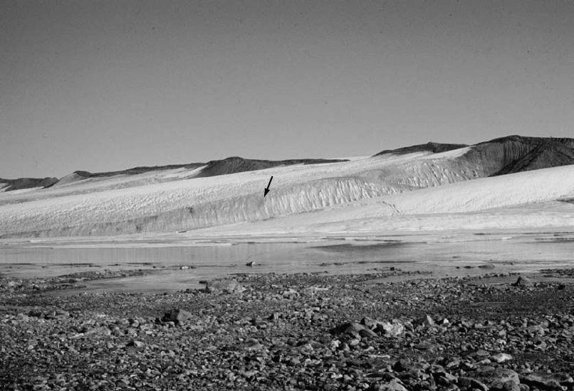
100 The velocity ﬁeld in a glacier

Figure 5.15. Thule–Bafﬁn moraines (on skyline) in one of the type areas, Thule

aq), Greenland. Note folding in foliation (sedimentary stratiﬁcation) in

superimposed ice in center of photograph. (From Hooke, 1970, Figure 8.

Reproduced with permission of the International Glaciological Society.)

example of the importance of drifting snow. The casual observer will

commonly be surprised to learn that although the crest of the moraine

in Figure 5.15 is several tens of meters above the margin, the till is usu-

ally no more than a meter or so thick. Beneath the till is dirty ice with

quite variable debris concentrations. The dirt in the ice is typically seg-

regated into laminae or folia, millimeters in thickness, that dip steeply

upglacier (Figure 5.16b). The sediment content of the dirt-bearing folia

is normally only a few percent. Layers of clast-supported frozen till,

sometimes exceeding1minthickness, are also present. The wedge of

ice downglacier from the moraine is clean. It is too thin to ﬂow at an

appreciable rate, and is frozen to its bed, preventing sliding. The low

ﬂow rate, in conjunction with the observed dip of the foliation, led to the

mistaken impression that the foliation planes were shear planes, and that

the dirty ice was actively shearing over the wedge of clean ice in such a

way that debris, entrained at the bed, was carried to the surface on these

planes.