Hjorth-Jensen M. Computational Physics

Подождите немного. Документ загружается.

Chapter 7

Numerical interpolation, extrapolation and

ﬁtting of data

7.1 Introduction

Numerical interpolation and extrapolation is perhaps one of the most used tools in numerical

applications to physics. The often encountered situation is that of a function

at a set of points

where an analytic form is missing. The function may represent some data points

from experiment or the result of a lengthy large-scale computation of some physical quantity

that cannot be cast into a simple analytical form.

We may then need to evaluate the function at some point within the data set , but

where differs from the tabulated values. In this case we are dealing with interpolation. If is

outside we are left with the more troublesomeproblem of numerical extrapolation. Below we will

concentrate on two methods for interpolation and extrapolation, namely polynomial interpolation

and extrapolation and the qubic spline interpolation approach.

7.2 Interpolation and extrapolation

7.2.1 Polynomial interpolation and extrapolation

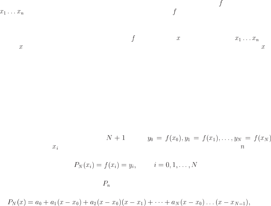
Let us assume that we have a set of

points

where none of the values are equal. We wish to determine a polynomial of degree so that

(7.1)

for our data points. If we then write

on the form

(7.2)

100

CHAPTER 7. NUMERICAL INTERPOLATION, EXTRAPOLATION AND FITTING

OF DATA

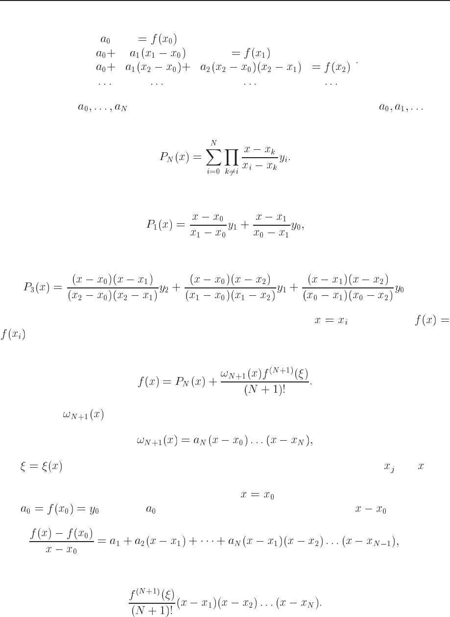
then Eq. (7.1) results in a triangular system of equations

(7.3)

The coefﬁcients

are then determined in a recursive way, starting with .

The classic of interpolation formulae was created by Lagrange and is given by

(7.4)

If we have just two points (a straight line) we get

(7.5)

and with three points (a parabolic approximation) we have

(7.6)

and so forth. It is easy to see from the above equations that when

we have that

It is also possible to show that the approximation error (or rest term) is given by the second

term on the right hand side of

(7.7)

The function

is given by

(7.8)

and

is a point in the smallest interval containing all interpolation points and . The

algorithm we provide however (the code POLINT in the program library) is based on divided

differences. The recipe is quite simple. If we take

in Eq. (7.2), we then have obviously

that

. Moving over to the left-hand side and dividing by we have

(7.9)

where we hereafter omit the rest term

(7.10)

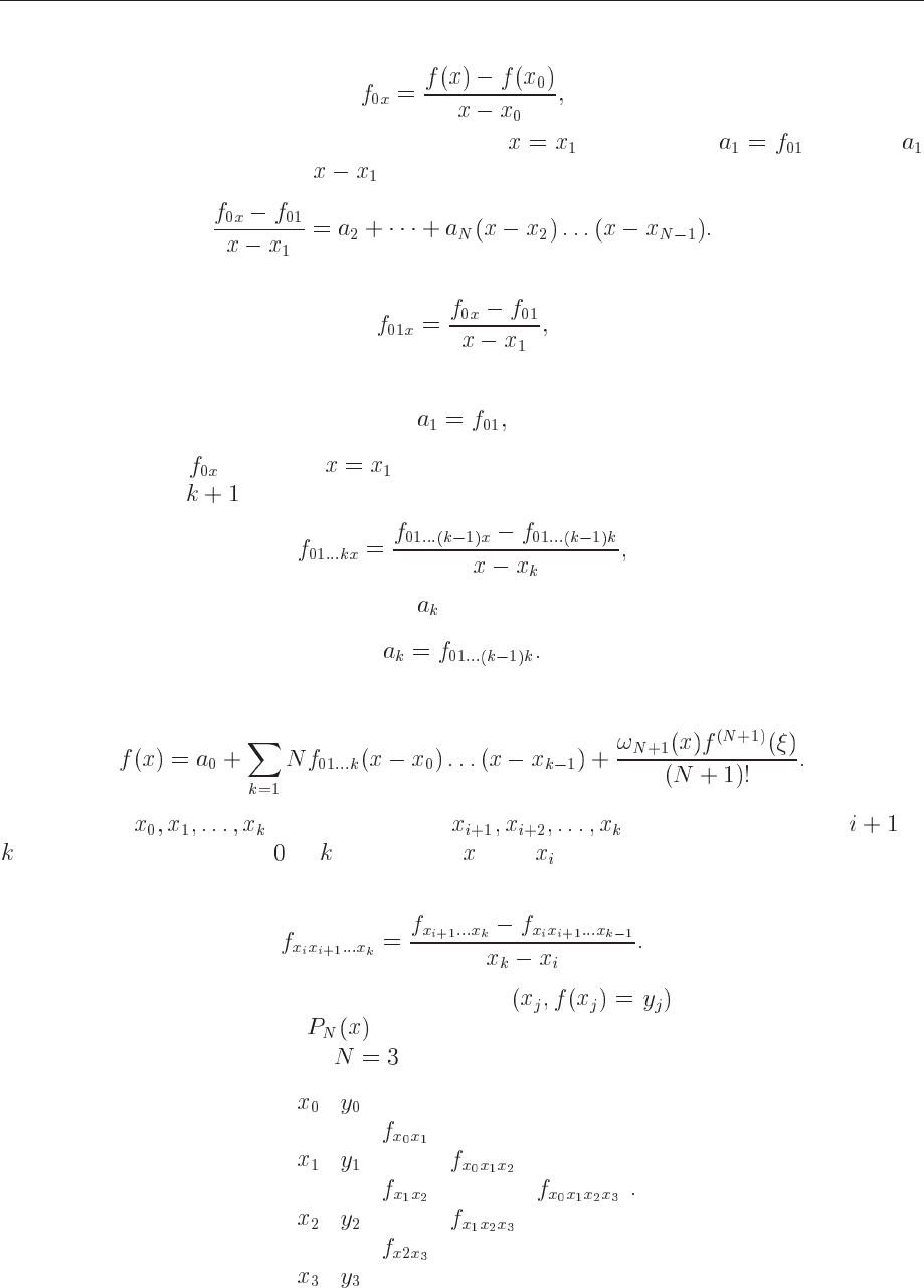
7.2. INTERPOLATION AND EXTRAPOLATION 101

The quantity

(7.11)

is a divided difference of ﬁrst order. If we then take

, we have that . Moving

to the left again and dividing by we obtain

(7.12)

and the quantity

(7.13)

is a divided difference of second order. We note that the coefﬁcient

(7.14)

is determined from

by setting . We can continue along this line and deﬁne the divided

difference of order as

(7.15)

meaning that the corresponding coefﬁcient is given by

(7.16)

With these deﬁnitions we see that Eq. (7.7) can be rewritten as

(7.17)

If we replace

in Eq. (7.15) with , that is we count from to

instead of counting from to and replace with , we can then construct the following

recursive algorithm for the calculation of divided differences

(7.18)

Assuming that we have a table with function values

and need to construct the

coefﬁcients for the polynomial . We can then view the last equation by constructing the

following table for the case where

(7.19)

102

CHAPTER 7. NUMERICAL INTERPOLATION, EXTRAPOLATION AND FITTING

OF DATA

The coefﬁcients we are searching for will then be the elements along the main diagonal. We

can understand this algorithm by considering the following. First we construct the unique poly-

nomial of order zero which passes through the point

. This is just discussed above.

Therafter we construct the unique polynomial of order one which passes through both and

. This corresponds to the coefﬁcient and the tabulated value and together with

results in the polynomial for a straight line. Likewise we deﬁne polynomial coefﬁcients for all

other couples of points such as

and . Furthermore, a coefﬁcient like

spans now three points, and adding together we obtain a polynomial which represents three

points, a parabola. In this fashion we can continue till we have all coefﬁcients. The function

POLINT included in the library is based on an extension of this algorithm, knowns as Neville’s

algorithm. It is based on equidistant interpolation points. The error provided by the call to the

function POLINT is based on the truncation error in Eq. (7.7).

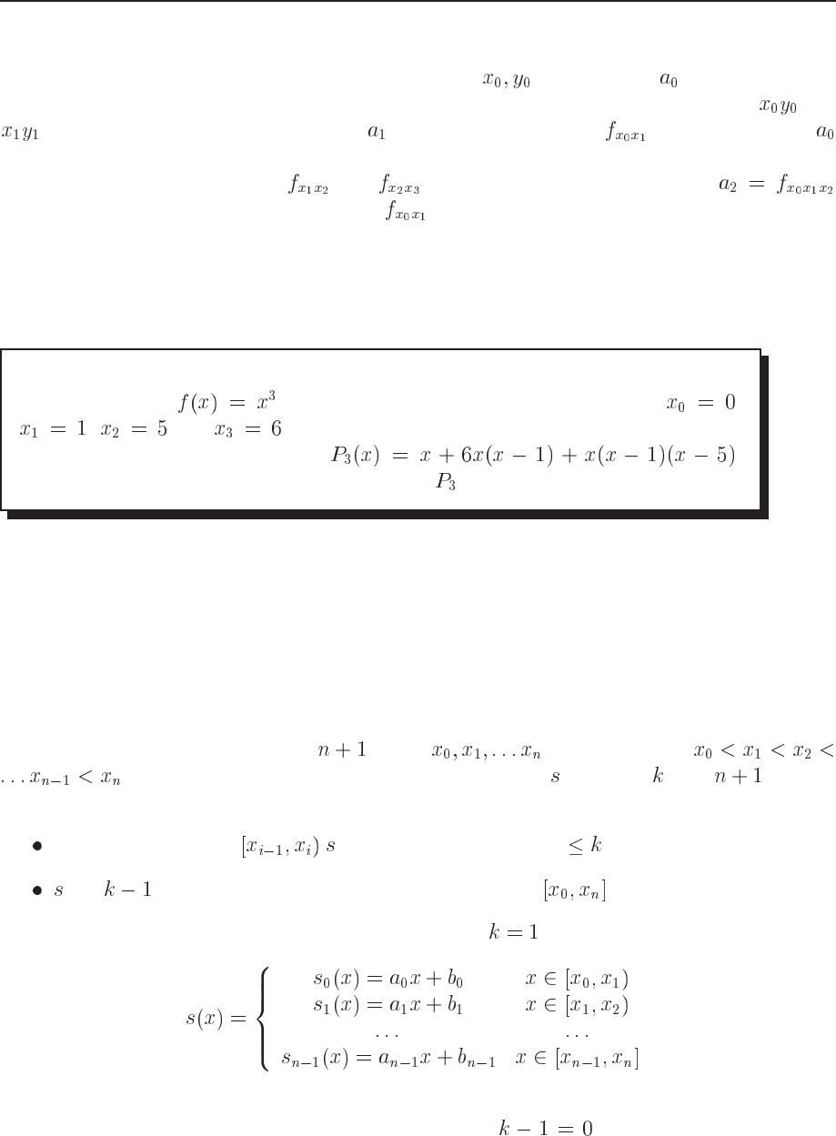
Exercise 6.1

Use the function

to generate function values at four points ,

, and . Use the above described method to show that the

interpolating polynomial becomes .

Compare the exact answer with the polynomial

and estimate the rest term.

7.3 Qubic spline interpolation

Qubic spline interpolation is among one of the mostly used methods for interpolating between

data points where the arguments are organized as ascending series. In the library program we

supply such a function, based on the so-called qubic spline method to be described below.

A spline function consists of polynomial pieces deﬁned on subintervals. The different subin-

tervals are connected via various continuity relations.

Assume we have at our disposal points arranged so that

(such points are called knots). A spline function of degree with knots is

deﬁned as follows

On every subinterval is a polynomial of degree .

has continuous derivatives in the whole interval .

As an example, consider a spline function of degree

deﬁned as follows

(7.20)

In this case the polynomial consists of series of straight lines connected to each other at every

endpoint. The number of continuous derivatives is then

, as expected when we deal

7.3. QUBIC SPLINE INTERPOLATION 103

with straight lines. Such a polynomial is quite easy to construct given points

and their corresponding function values.

The most commonly used spline function is the one with

, the so-called qubic spline

function. Assume that we have in adddition to the

knots a series of functions values

. By deﬁnition, the polynomials and are thence

supposed to interpolate the same point

, i.e.,

(7.21)

with

. In total we have polynomials of the type

(7.22)

yielding

coefﬁcients to determine. Every subinterval provides in addition the conditions

(7.23)

and

(7.24)

to be fulﬁlled. If we also assume that

and are continuous, then

(7.25)

yields

conditions. Similarly,

(7.26)

results in additional

conditions. In total we have coefﬁcients and equations to

determine them, leaving us with degrees of freedom to be determined.

Using the last equation we deﬁne two values for the second derivative, namely

(7.27)

and

(7.28)

and setting up a straight line between

and we have

(7.29)

and integrating twice one obtains

(7.30)

104

CHAPTER 7. NUMERICAL INTERPOLATION, EXTRAPOLATION AND FITTING

OF DATA

Using the conditions and we can in turn determine the constants

and resulting in

(7.31)

How to determine the values of the second derivatives and ? We use the continuity

assumption of the ﬁrst derivatives

(7.32)

and set

. Deﬁning we obtain ﬁnally the following expression

(7.33)

and introducing the shorthands

, , we

can reformulate the problem as a set of linear equations to be solved through e.g., Gaussian

elemination, namely

(7.34)

Note that this is a set of tridiagonal equations and can be solved through only

operations.

The functions supplied in the program library are and . In order to use qubic spline

interpolation you need ﬁrst to call

sp line ( double x [ ] , double y [ ] , int n , double yp1 , double yp2 , double

y2 [ ] )

This function takes as input and containing a tabulation

with together with the ﬁrst derivatives of at and , respectively.

Then the function returns

which contanin the second derivatives of at each

point . is the number of points. This function provides the qubic spline interpolation for all

subintervals and is called only once. Thereafter, if you wish to make various interpolations, you

need to call the function

s p l i n t ( double x [ ] , double y [ ] , double y2a [ ] , int n , double x , double

which takes as input the tabulated values and and the output y2a[0,..,n

- 1] from

. It returns the value corresponding to the point .

Chapter 8

Numerical integration

8.1 Introduction

In this chapter we discuss some of the classic formulae such as the trapezoidal rule and Simpson’s

rule for equally spaced abscissas and formulae based on Gaussian quadrature. The latter are more

suitable for the case where the abscissas are not equally spaced. The emphasis is on methods for

evaluating one-dimensional integrals. In chapter 9 we show how Monte Carlo methods can be

used to compute multi-dimensional integrals. We end this chapter with a discussion on singular

integrals and the construction of a class for integration methods.

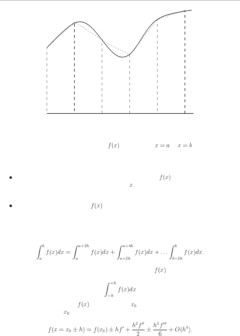
The integral

(8.1)

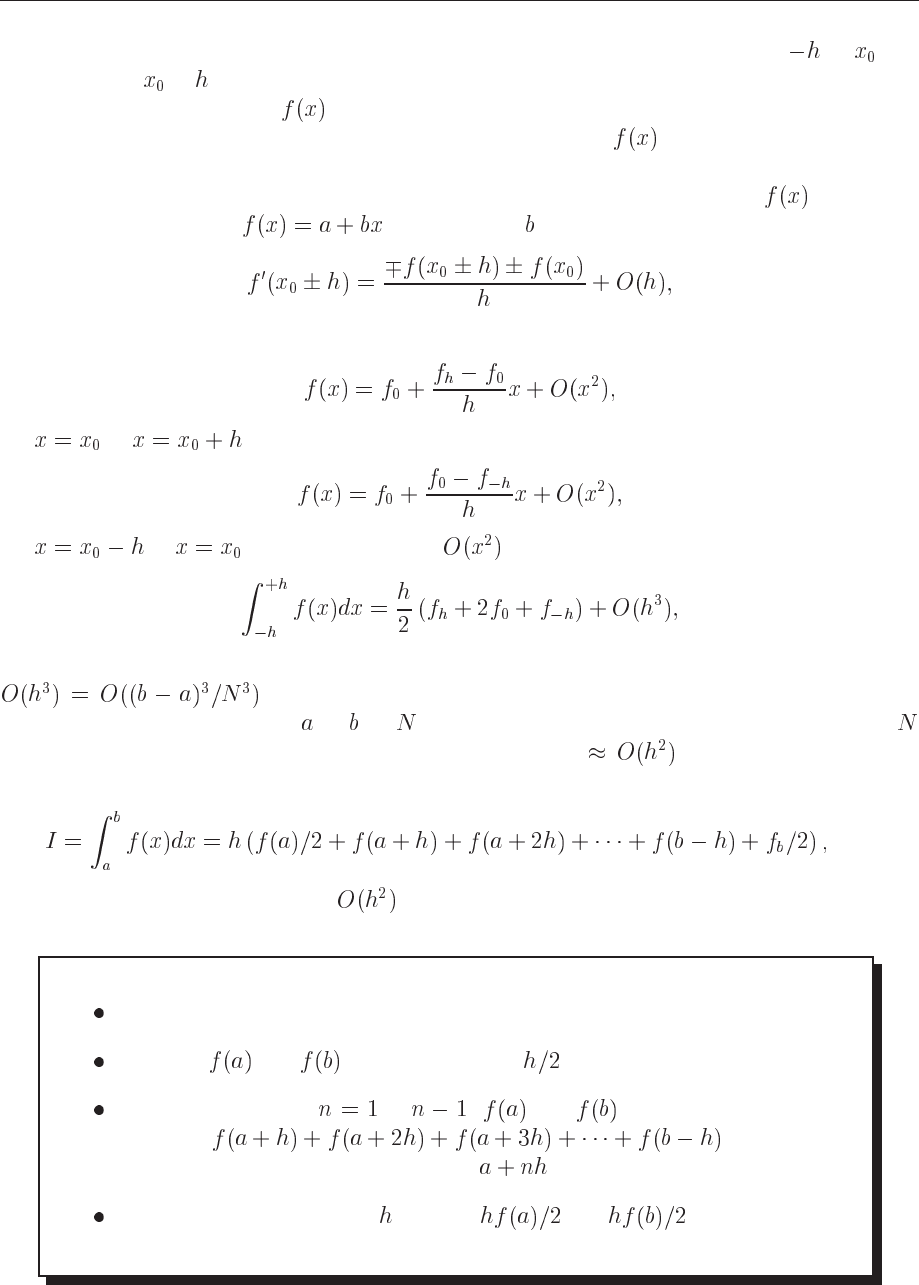
has a very simple meaning. If we consider Fig. 8.1 the integral

simply represents the area

enscribed by the function

starting from and ending at . Two main methods will

be discussed below, the ﬁrst one being based on equal (or allowing for slight modiﬁcations) steps

and the other on more adaptive steps, namely so-called Gaussian quadrature methods. Both main

methods encompass a plethora of approximations and only some of them will be discussed here.

8.2 Equal step methods

In considering equal step methods, our basic tool is the Taylor expansion of the function

around a point and a set of surrounding neighbouring points. The algorithm is rather simple,

and the number of approximations unlimited!

Choose a step size

where is the number of steps and and the lower and upper limits of integration.

105

106 CHAPTER 8. NUMERICAL INTEGRATION

a a+h a+2h a+3h a+4h b

Figure 8.1: Area enscribed by the function starting from to . It is subdivided in

several smaller areas whose evaluation is to be approximated by the techniques discussed in the

text.

Choose then to stop the Taylor expansion of the function at a certain derivative. You

should also choose how many points around are to be included in the evaluation of the

derivatives.

With these approximations to perform the integration.

Such a small measure may seemingly allow for the derivation of various integrals. To see this,

let us brieﬂy recall the discussion in the previous section and especially Fig. 3.1. First, we can

rewrite the desired integral as

(8.2)

The strategy then is to ﬁnd a reliable Taylor expansion for

in the smaller sub intervals.

Consider e.g., evaluating

(8.3)

where we will Taylor expand

around a point , see Fig. 3.1. The general form for the

Taylor expansion around

goes like

8.2. EQUAL STEP METHODS 107

Let us now suppose that we split the integral in Eq. (8.3) in two parts, one from to and

the other from

to . Next we assume that we can use the two-point formula for the derivative,

that is we can approximate in these two regions by a straight line, as indicated in the

ﬁgure. This means that every small element under the function looks like a trapezoid, and

as you may expect, the pertinent numerical approach to the integral bears the predictable name

’trapezoidal rule’. It means also that we are trying to approximate our function

with a ﬁrst

order polynomial, that is

. The constant is the slope given by ﬁrst derivative

and if we stop the Taylor expansion at that point our function becomes,

(8.4)

for

to and

(8.5)

for

to . The error goes like . If we then evaluate the integral we obtain

(8.6)

which is the well-known trapezoidal rule. Concerning the error in the approximation made,

, you should note the following. This is the local error! Since we

are splitting the integral from

to in pieces, we will have to perform approximately

such operations. This means that the global error goes like . To see that, we use the

trapezoidal rule to compute the integral of Eq. (8.1),

(8.7)

with a global error which goes like

. It can easily be implemented numerically through the

following simple algorithm

Choose the number of mesh points and ﬁx the step.

calculate and and multiply with

Perform a loop over to ( and are known) and sum up

the terms . Each step in

the loop corresponds to a given value .

Multiply the ﬁnal result by and add and .

108 CHAPTER 8. NUMERICAL INTEGRATION

A simple function which implements this algorithm is as follows

double t r apez o i dal_ r u l e ( double a , double b , int n , double ( func ) (

double ) )

{

double trapez_sum ;

double fa , fb , x , step ;

int j ;

step =(b a ) / ( ( double ) n ) ;

fa =( func ) ( a ) / 2 . ;

fb =( func ) ( b ) / 2 . ;

trapez_sum =0. ;

for ( j =1; j <= n 1; j ++){

x= j step +a ;

trapez_sum +=( func ) ( x ) ;

}

trapez_sum =( trapez_sum +fb+fa ) step ;

return trapez_sum ;

} / / end trape zoida l_ ru le

The function returns a new value for the speciﬁc integral through the variable trapez_sum. There

is one new feature to note here, namely the transfer of a user deﬁned function called func in the

deﬁnition

void trap e z o ida l _ r ule ( double a , double b , int n , double trapez_sum ,

double ( func ) ( double ) )

What happens here is that we are transferring a pointer to the name of a user deﬁned function,

which has as input a double precision variable and returns a double precision number. The

function trapezoidal_rule is called as

t ra p e zoid a l _ rul e (a , b , n , & trapez_sum , & myfunction )

in the calling function. We note that a, b and n are called by value, while trapez_sum and the

user deﬁned function my_function are called by reference.

Instead of using the above linear two-point approximation for

, we could use the three-point

formula for the derivatives. This means that we will choose formulae based on function values

which lie symmetrically around the point where we preform the Taylor expansion. It means also

that we are approximating our function with a second-order polynomial

The ﬁrst and second derivatives are given by

(8.8)

and

(8.9)