Glusker J.P., Trueblood K.N. Crystal Structure Analysis: A Primer

Подождите немного. Документ загружается.

(a)

(b)

(1) (2)

(3)

(4)

(1) Section x=0.42

Atom B in incorrect position on x=0.42 (position A)

Atom B in correct position on x=0.042 (position B)

(3) Section x=0.42

(4) Section x=0.042 (atom B)

(2) Section x=0.042

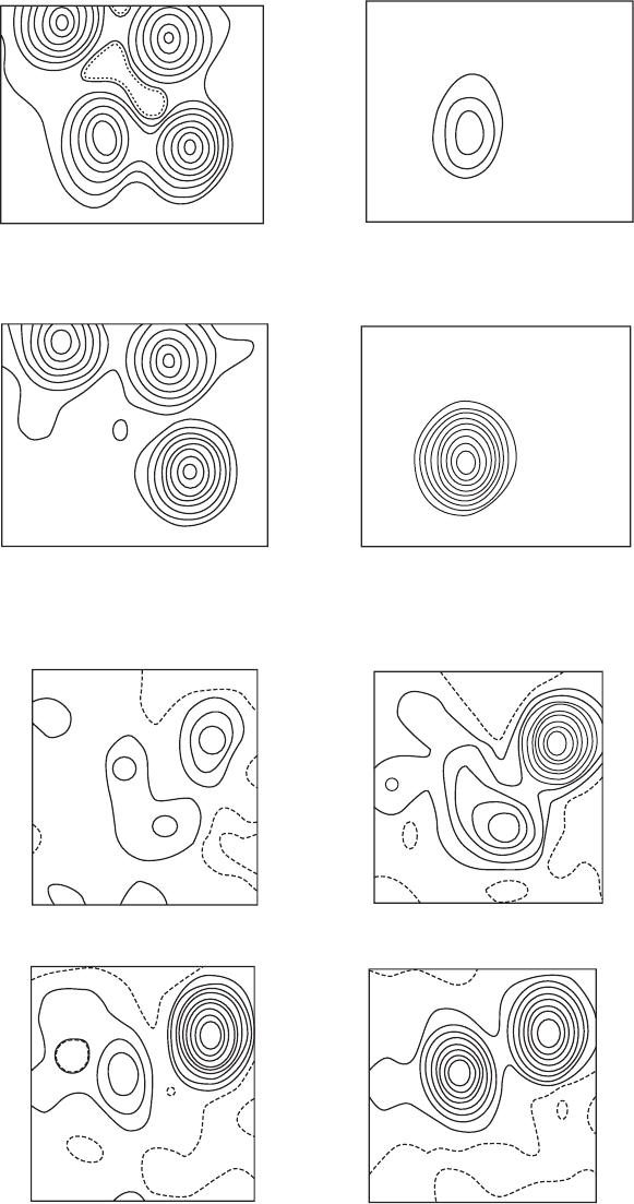
Fig. 11.1 Fourier maps phased with partially incorrect trial structures.

Fourier methods 169

map calculated with observed structure amplitudes and computed phase

angles will contain a blend of the true structure (from the structure

amplitudes) with the trial structure (from the calculated phases). If

the trial structure contains most of the atoms of the true structure,

at or near their correct positions, the resulting electron-density map

will contain peaks representing the trial structure, but, additionally, at

other sites, peaks representing atoms that were omitted from the trial

structure but that are really present. Conversely, if an atom in the trial

structure has been incorrectly chosen, the corresponding peak in the

electron-density map will usually be signiﬁcantly lower than normal,

so that its location will be questionable. Finally, if an atom was put

into the calculation near, but not at, its correct position, the resulting

peak in the electron-density map will usually have moved a slight

amount from the input position towards (but not usually as far as) the

correct position. Examples of these effects for a noncentrosymmetric

structure are shown in Figure 11.1. In centrosymmetric structures, the

phase angles are either 0

◦

or 180

◦

and a slight error in the structure

may not have a large effect on most phase angles. Therefore, a map

computed with observed |F ( hkl )| values and computed phase angles

may be almost correct even if the model used was slightly in error.

However, with noncentrosymmetric structures, for which the phase

angles may have any value from 0

◦

to 360

◦

, there will be at least small

errors in most of the phases, and consequently the calculated electron-

density map will be weighted more in the direction of the trial structure

used to calculate the phases than it would be if the structure were

centrosymmetric.

It is usual, when most or all of the trial structure is known, to compute

difference maps rather than normal electron-density maps. For difference

maps, the coefﬁcients for the calculation are (|F

|−|F

|) and the phase

(a) The effect of an atom in the wrong position. This example is from a noncentrosymmet-

ric structure. In (1), one atom, B, was inadvertently included (an input typographi-

cal error) at the wrong position (marked by an A) in the structure factor calculation.

The electron-density map phased with this incorrect structure contains a peak at

the wrong position, but this peak is lower in electron density than the others near

it. A small peak occurs in the correct position, B, shown in (2), although none was

introduced there in the phasing. Corresponding sections of a correctly phased map

are shown in (3) and (4); the spurious “atom” at A above has disappeared and the

correct peak, B, is now a pronounced one.

(b) The effect of an atom near but not at the correct position. The appearance of a partic-

ular section in successive electron-density maps is shown as the structure used

for phasing becomes more nearly correct. The map (1) was computed from the

positions of two heavy atoms (positions not shown) and from this the location of

atom X was correctly (as it turned out) deduced. But in (2) an atom was incorrectly

placed at P; it can be seen that the peak for this atom is elongated in the direction

of the correct position, Q. In (3) only atom X (of P, Q, and X) was included in the

phasing and peak Q now is more clearly revealed. In (4) the peak at Q is now

established as correct. A total of 2, 62, 54, and 68 atoms out of 73 were used in the

phasing of maps (1), (2), (3), and (4), respectively.

From Hodgkin et al., 1959, p. 320, Figures 8 and 9.

170 Reﬁnement of the trial structure

angles are those computed for the trial structure. The difference map

is thus the difference of an “observed” and a “calculated” map (both

with “calculated” phases). In this map a positive region implies that

not enough electrons were put in that area in the trial structure, while

a negative region suggests that too many electrons were included in

that region in the trial structure. For example, if an atom is included in

the trial structure with too high an atomic number, a trough appears

at the corresponding position; if it is included (at the correct position)

with too low an atomic number or omitted entirely, a peak appears.

Hydrogen atoms can be located from difference maps calculated from

a trial structure that includes all the heavier atoms present (see Fig-

ure 11.2), although often hydrogen atoms are put at geometrically cal-

culated positions and then reﬁned. Another use of difference maps is in

macromolecular structure determination, to locate the binding sites of

inhibitors, substrates, or products.

Figure 11.3 shows some examples of further uses of difference maps

for reﬁnement of parameters. If an atom has been included near but

not at the correct position, the location at which it was input will lie

in a negative region, with a positive region in the direction of the

correct position. The amount of the shift needed to move the atom to

the correct position is indicated by the slope of the contours between the

negative and positive regions. If an atom is left out of the trial structure

(as in “omit maps”) it will appear in the correct position as a peak, pro-

vided, of course, that the phase angles used in computing the electron-

density map are approximately correct. If an atomic displacement factor

is too small in the calculated trial structure, a trough will appear at the

atomic position because the electrons in that atom have been assumed

in the trial structure to be conﬁned to a smaller volume than in fact they

are, and hence to have too high a total electron density. Similarly, if the

atomic displacement factor is too large in the trial structure, a peak will

appear in the difference map. If the atom vibrates anisotropically, that

is, different amounts in different directions, but has been assumed to be

isotropic, peaks will occur in directions of greater motion and troughs

in directions of lesser motion. In summary, if there is a positive area in a

difference map, consider adding more electron density at that position;

a negative area indicates too much electron density at that location in

the trial structure.

The process of Fourier reﬁnement can be adapted for automatic

operation with a high-speed computer. Instead of evaluating the elec-

tron density at the points of a ﬁxed lattice, we calculate it, together

with its ﬁrst and second derivatives, at the positions assumed for

the atomic centers at this stage. The shifts in the atomic posi-

tions

and temperature-factor parameters can then be derived from

The shift required in x is

ƒx =

−∂ƒÒ

∂x

∂

∂x

−(gradient of difference Fourier at x

)

(curvature of electron density at x

)

where x

is the input position.

the slopes and the curvatures in different directions. When this

differential-synthesis method is used, it is normally applied to the

difference density. In fact, however, the method is used much less

extensively than least-squares reﬁnement, for the latter is somewhat

more convenient for computer application and has the advantage

Fourier methods 171

0.00

0.50

H(7)

H(1)

H(5)

H(8)

H(2)

H(4)

H(6)

H(3)

0.50

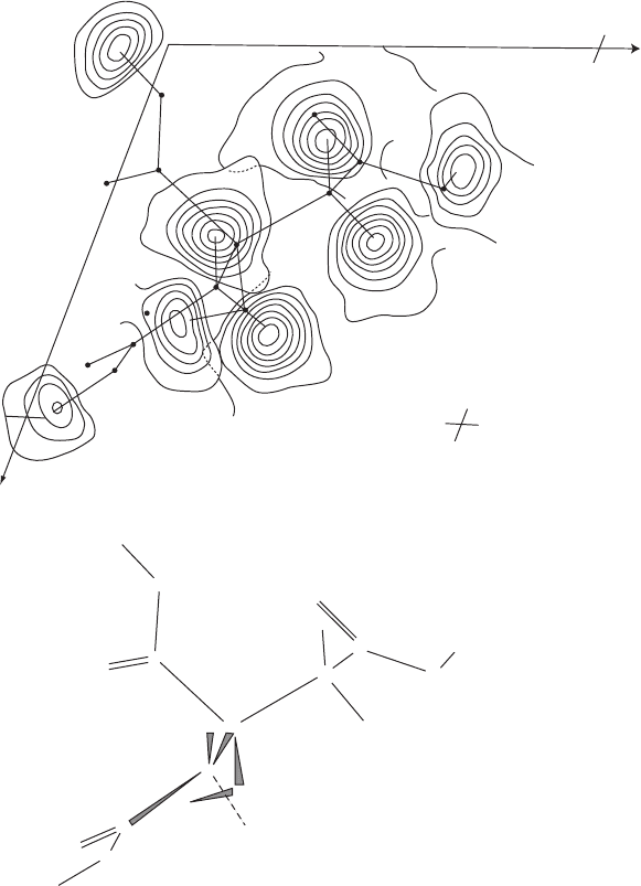
Fig. 11.2 Hydrogen atoms found from a difference map.

This is a composite map of sections of a difference map for a monoclinic structure, anhydrous citric acid, viewed down b. Eight sections

containing hydrogen atoms are shown here. The contour interval is 0.1 electrons per cubic Å; the zero contour is omitted. Solid circles

show the ﬁnal positions of the heavier atoms that were used in the phase-angle calculation. Peaks occur in the map at positions in which

not enough electron density has been included in the structure factor calculation, and thus at the positions of hydrogen atoms omitted

from the phase-angle calculation. The molecular formula is shown below the map, on the same scale and in the same orientation.

From Glusker et al., 1969, Acta Crystallographica B25, p. 1066, Figure 1.

of a statistically sounder weighting scheme for the experimental

observations.

One of the best criteria of a good structure determination is a ﬂat

difference map at the end of the reﬁnement (because now the values

of the observed and calculated structure amplitudes are approximately

172 Reﬁnement of the trial structure

Move atom

(a) (b)

calc

obs

∆

r = (r

obs

–r

cale

)

∆

r = (r

obs

–r

calc

)

calc

iso

too high)

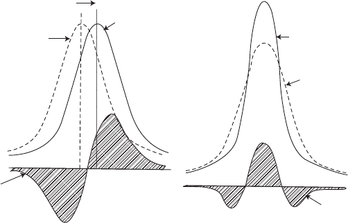
Fig. 11.3 Reﬁnement by difference maps.

A difference map (the difference between the observed and calculated electron density, Ò

obs

− Ò

calc

) may be used to reﬁne atomic

positions and temperature factors. In a difference map a peak (a region of positive electron density) implies that not enough electron

density was included in the model at that position, and a trough (a region of negative electron density) implies the opposite.

(a) An error in the position of an atom. The peak in Ò

calc

shows the approximate position used in the calculation of structure factors.

The peak in Ò

obs

is nearer to the correct position. Therefore, the assumed atomic position should be moved (to the right) in the

direction of the positive peak in the difference map.

(b) Incorrect atomic displacement parameter. If the displacement parameter exponent is too high in the model used to phase the map, the

atom is vibrating through too large a volume. A peak surrounded by a region of negative density occurs at the atomic position,

indicating that the exponent should be decreased to give a higher and narrower peak (and thus B should be decreased).

equal). It is possible to have a good average agreement of |F

| and |F

and thus a low discrepancy index, R, and yet to have many (|F

|−|F

values contributing to a peak or trough in a given area of the map,

indicating some error in the structure. Therefore, at the end of every

structure determination, a difference map should be calculated and

scanned for any peaks.

One question that always arises in discussions of Fourier reﬁnement

is: How good must the trial structure be, or how nearly correct must

the phases be, for the process to converge? This question cannot be

answered precisely. For an ordinary small-molecule structure analysis,

if most of the atoms included are within about 0.3 Å (approximately

half their radius) of their correct sites, then a few that are farther away

and even one or two that may be wholly spurious can be tolerated.

When the initial phases are poor, the ﬁrst approximations to the electron

density will contain much false detail (as illustrated in Figures 9.8 and

11.1b), together with peaks at or near the correct atomic positions. The

sorting of the real from the spurious is difﬁcult, especially with noncen-

trosymmetric structures; experience, chemical information, and a sound

knowledge of the principles of structural chemistry are all desirable,

and a good deal of caution is essential. A very astute or fortunate crys-

tallographer may be able to recognize portions of a molecule of known

The method of least squares 173

structure in a map produced from an extremely poor trial structure, but

such perspicacity is uncommon.

Most investigators currently view electron-density and difference

maps on a computer screen. There are several mouse-driven three-

dimensional interactive programs such as O (Jones et al., 1991) and

COOT (Emsley and Cowtan, 2004) that show electron densities as three-

dimensional wire-frame entities. These can be rotated by the user to

better view them, and a diagram of a three-dimensional trial structure

can be overlaid on them. Some reﬁnement can even take place at the

computer screen as the trial structure diagram is moved to best ﬁt the

map. When the user is satisﬁed with the ﬁt, the program will then

generate the atomic coordinates of the new and better position of the

model and these coordinates can be further reﬁned.

The method of least squares

The method of least squares, ﬁrst used by Legendre (1805), is a common

technique for ﬁnding the best ﬁt of a particular assumed model toasetof

experimental data when there are more experimental observations than

parameters to be determined. Parameters for the assumed model are

improved by this method by minimizing the sum of the squares of the

deviations between the experimental quantities and the values of the

same quantities calculated with the derived parameters of the model.

The method of least squares is often used to calculate the best straight

line through a series of points, when it is known that there is an experi-

mental error (assumed random) in the measurement of each point. The

equation for a line may be calculated such that the sum of the squares

of the deviations from the line is a minimum. Of course, if the points,

which were assumed to lie on a straight line, actually lie on a curve

(described very well by a nonlinear equation), the method will not tell

what this curve is, but will approximate it by a straight line as best it

may. It is possible to “weight” the points; that is, if one measurement

is believed to be more precise than the others, then this measurement

may, and indeed should, be given higher weight than the others. The

weight w(hkl) assigned to each measurement is inversely proportional

to its precision, that is, the square of the standard uncertainty (formerly

known as the estimated standard deviation).

The least-squares method has been extended to the problem of ﬁtting

the observed diffraction intensities to calculated ones (Hughes, 1946),

and has been for more than six decades by far the most commonly

used method of structure reﬁnement, although this practice has not

been without serious criticism.

Just as in a least-squares ﬁt of data to a

These criticisms are based in part on the

fact that the theory of the least-squares

method is founded on the assumption

that the experimental errors in the data

are normally distributed (that is, follow a

Gaussian error curve), or at least that the

data are from a population with ﬁnite sec-

ond moments. This assumption is largely

untested with most data sets. Weighting

of the observations may help to alleviate

the problem, but it depends on a knowl-

edge of their variance, which is usually

assumed rather than experimentally mea-

sured. For a discussion of some of these

points, see Dunitz’s discussion of least-

squares methods (Dunitz, 1996).

straight line (a two-parameter problem), the observed data are ﬁtted to

those calculated for a particular assumed model. If we let ƒ|F (hkl)| be

the difference in the amplitudes of the observed and calculated struc-

ture factors, |F

|−|F

|, and let the standard uncertainty of the experi-

mental value of F

(hkl)

be [1/w(hkl)], then, according to the theory of

174 Reﬁnement of the trial structure

errors, the best parameters of the model assumed for the structure are

those corresponding to the minimum value of the quantity

†

The equations can be formulated with

| rather than |F |, so that the equation

parallel to Eqn. (11.1) then becomes

Q = w(hkl)[ƒ|F

(hkl)|]

Most crystallographers prefer reﬁnement

that involves F

for a variety of reasons,

including ease of reﬁning twinned struc-

tures, calculating weights for the least-

squares reﬁnement, and dealing with

weak Bragg reﬂections (which may have

negative values of F

from the nature of

the measurement process).

Q = w(hkl)[ƒ|F(hkl)

(11.1)

in which the sum is taken over all unique diffraction maxima. In an

analysis of the equations that deﬁne F

, the effects of small changes

in the atomic parameters are considered, and changes are f ound that

will difference between F

and F

[and thus the sum in Eqn. (11.1)].

Since even the problem of ﬁtting data to a two-parameter straight line

involves much calculation, this method requires a high-speed, large-

memory computer.

The variable parameters that are used in the minimization of Q in

Eqn. (11.1) normally include an overall scale factor for the experimental

observations; the atomic position parameters x, y,andz for each atom,

j; and the atomic displacement parameters for each atom, which may

number as many as six.

‡

Occasionally, when disorder is present, occu-

‡

These six vibration parameters, different

for each atom j, are symbolized in vari-

ous ways (see Chapter 12). Here we rep-

resent them as b

, b

,and

, with sometimes an additional sub-

script to denote the atom j. As mentioned

later, more parameters may be needed to

describe the atomic motion in extreme cir-

cumstances.

pancy factors (varying from 0 to 1, and perhaps correlated with those

of other atoms) may be reﬁned for selected atoms. Thus in a general case

there may be as many as (9N + 1) or even a few more parameters to be

reﬁned for a structure with N independent atoms.

If the total number of parameters to be reﬁned is p, then the mini-

mization of Eqn. (11.1) involves setting the derivatives of Q with respect

to each of these parameters equal to zero. This gives p independent

simultaneous equations. The derivatives of Q are readily evaluated.

Clearly, at least p experimental observations are needed to deﬁne the p

parameters, but, in fact, since the observations usually have signiﬁcant

experimental uncertainty, it is desirable that the number of observa-

tions, m, exceeds the number of variables by an appreciable factor. In

most practical cases with three-dimensional X-ray data, m/p is of the

order of 5 to 10, so that the equations derived from Eqn. (11.1) are

greatly overdetermined.

Unfortunately, the equations derived from Eqn. (11.1) are by no

means linear in the parameters, since they involve trigonometric and

exponential functions, whereas the straightforward application of the

method of least squares requires a set of linear equations. If area-

sonable trial structure is available, then it is possible to derive a set

of linear equations in which the variables are the shifts from the trial

parameters, rather than the parameters themselves. This is done by

expanding in a Taylor series about the trial parameters, retaining only

the ﬁrst-derivative terms on the assumption that the shifts needed are

sufﬁciently small that the terms involving second- and higher-order derivatives

are negligible:

∂

∂x

ƒx

∂

∂y

ƒy

+ ···+

∂

∂b

33,n

ƒb

33,n

(11.2)

The validity of this assumption depends on the closeness of the trial

structure to the correct structure. If conditions are unfavorable, and

Eqn. (11.2) is too imprecise, the process may sometimes converge to

The method of least squares 175

a false minimum rather than to the minimum corresponding to the

correct solution or may not converge at all. Thus this method of reﬁne-

ment also depends for its success on the availability at the start of a

reasonably good set of phases—that is, a good trial structure. Since the

linearization of the least-squares equations makes them only approx-

imate, several cycles of reﬁnement are needed before convergence is

achieved. However, the linear approximation becomes better as the

solution is approached because the neglected higher-derivative terms,

which involve high powers of the discrepancies between the approx-

imate and true structures, become negligible as these discrepancies

become small.

It is often desirable in a least-squares reﬁnement to introduce various

constraints or restraints on the atomic parameters to make them satisfy

some speciﬁc criteria, usually geometrical. Constraints are limits on

the values that parameters in a least-squares reﬁnement may take. For

example, they may relate two or more parameters, or may assign ﬁxed

values to certain parameters. As a result they reduce the number of

independent parameters to be reﬁned and are mathematically rigid

with no standard uncertainty. For example, suppose that the structure is

disordered in some way, or that the available diffraction data are of lim-

ited resolution. The individual atomic positions obtained by the usual

least-squares process for some of the atoms will then have relatively

high standard uncertainties and the geometrical parameters derived

from these positions may not be of high signiﬁcance. If geometrical

constraints are introduced—for example, constraining a phenyl ring to

be a regular hexagon of certain dimensions, or merely ﬁxing certain

bond lengths or bond angles or torsion angles within a particular range

of values—the number of parameters to be reﬁned will be signiﬁcantly

reduced and the reﬁnement process accelerated. By contrast, restraints

are assumptions that are treated like additional data that need to be

reﬁned against. For example, a phenyl group would be described as an

“approximately regular hexagon” with a standard uncertainty within

which it is supposed to be reﬁned. Constraints remove parameters and

restraints add data.

If the trial model used in a least-squares reﬁnement is incorrect or

partially incorrect, there are almost always indications that this is so.

The discrepancy index R may not drop to an acceptable value, and

the parameters may show certain anomalies. For example, if a false

atom has inadvertently been included in the initial trial structure, it

may move to a chemically unreasonable position, perhaps too close to

another atom, and its temperature factor will increase strikingly to a

value far higher than that normally encountered for any real atom. This

corresponds physically to a very high vibration amplitude—that is, a

smearing of the atom throughout the unit cell, an almost infallible sign

that there is no atom in the actual structure at the position assumed in

the trial structure.

At the conclusion of any least-squares reﬁnement process, it is always

wise to calculate a difference Fourier synthesis. If it is zero everywhere,

176 Reﬁnement of the trial structure

within experimental error, then the least-squares procedure is a reason-

able one. If it is not, and the peaks in it are not attributable to light

atoms that have been left out of the structure factor calculations or to

some other understandable defect of the model, then it is distinctly

possible that the least-squares procedure may have converged to a false

minimum because the initial approximation (the trial structure) was not

sufﬁciently good. Another plausible trial structure must be sought and

reﬁnement tried again.

The maximum likelihood method

Maximum likelihood estimation is an increasingly commonly

employed statistical method that is used to reﬁne a statistical model

to experimental data, and thereby provide improved estimates of the

parameters of this model (Murshudov et al., 1997; Terwilliger, 2000).

It deals in conditional probability distributions, that is, probabilities

that are conditional upon additional variables, and aims to maximize

their likelihoods. For example, if we know that the probability of data

A is dependent upon model B, we can ﬁnd the likelihood of model

B given the data A. Stephen Stigler compares maximum likelihood

to the choice that prehistoric men made of “where and how to hunt

and gather,” that is, experience and acute observation which indicates

how best to do something (Stigler, 2007). The likelihood function

for macromolecular structures is proportional to the conditional

distribution of experimental data when the parameters are known.

The conditional probability distributions for each Bragg reﬂection are

multiplied together and the result is the joint conditional probability

distribution. This includes the experimental data plus any phase

information and any experimental standard uncertainties that may

be available. The aim of the method is to ﬁnd those values of the

parameters that make the observed data most likely. The necessary

equations are contained in the program REFMAC (Vagin et al., 2004),

which will minimize atomic parameters to satisfy either a maximum

likelihood or a least-squares residual. The method has been used

with great success, and, if the data have been measured to very high

resolution, approaches least squares as a good reﬁnement method.

The correctness of a structure

What assurance is there that the changes suggested by difference maps,

least-squares methods, or maximum likelihood estimations are correct?

Are the suggested changes really improvements that will make the

trial structure more nearly resemble the actual distribution of scatter-

ing matter in the crystal? In fact, if the experimenter is injudicious

or unfortunate, some changes may actually make the model worse,

since an image formed with incorrect phases will always contain false

The correctness of a structure 177

detail—for example, peaks that may seem to suggest atoms but that

really arise from errors in the phases. If the model is altered in a

grossly incorrect way (or if it was inadequate in the ﬁrst place), the

“reﬁnement” process may converge to a quite incorrect solution. What

then are the criteria for assessing the likely correctness of a structure

that has been determined by the reﬁnement of approximate phases?

There are no certain tests, but the most helpful general criteria are

the following. (A number of erroneous structures have been reported

because of inadequate attention to these criteria.)

(1) The agreement of the individual observed structure factor ampli-

tudes |F

| with those calculated for the reﬁned model should be

comparable to the estimated precision of the experimental mea-

surements of the |F

|. As stressed in Chapter 6, the discrepancy

index, R [Eqn. (6.9)], is a useful but by no means deﬁnitive index

of the reliability of a structure analysis.

(2) A difference map phased with the ﬁnal parameters of the reﬁned

structure should reveal no ﬂuctuations in electron density greater

than those expected on the basis of the estimated precision of the

electron density.

(3) Any anomalies in the molecular geometry and packing, or other

derived quantities—for example, abnormal bond distances and

angles, unusually short nonbonded intramolecular or intermolec-

ular distances, and the like—should be scrutinized with the great-

est care and regarded with some skepticism. They may be quite

genuine, but if so they should be interpretable in terms of some

unusual properties of the crystal or the molecules and ions in it.

If writers of crystallographic papers have done their work properly,

the information needed for a reader to assess the precision and accuracy

of the reported results will be given. The precision of an experimen-

tal result, usually expressed in terms of its standard uncertainty, is

a measure of the reproducibility of the observed value if the exper-

iment were to be repeated. Accuracy, on the other hand, gives the

deviation of a measurement from the value accepted as true (if that is

known). The standard uncertainties of the various observed results—

distances, angles, and so on—can be estimated by statistical methods,

using as a basis the estimated errors of the prime experimental quan-

tities, the intensities and directions of the diffracted radiation and the

instrumental parameters of the equipment used. The basic assumption

involved in the estimation of standard uncertainties is that ﬂuctuations

in observed quantities are due solely to random errors, which implies

that the ﬂuctuations are about an average value that agrees with the

“true value.” However, it is very important to recognize that there

may be systematic errors, too, arising from failure to correct for various

effects, which may be either known—for example, the effect of absorp-

tion on the intensities—or unknown—for example, inadequacies of the

model because of lack of knowledge of the way in which molecular

motion occurs in the crystal. Uncorrected systematic errors can cause