Ellwanger U. From the Universe to the Elementary Particles: A First Introduction to Cosmology and the Fundamental Interactions

Подождите немного. Документ загружается.

Chapter 10

The Standard Model of Particle Physics

The current version of the Standard Model of particle physics is based on only a few

elementary particles: six quarks and six leptons, the gauge ﬁelds responsible for the

interactions, and the still sought-after Higgs boson. The fundamental interactions

relevant for particle physics are the electromagnetic, strong, and weak interactions.

This chapter summarizes the properties of the elementary particles, the aspects shared

by the fundamental interactions and where they differ, and the open questions left

unanswered by the Standard Model.

10.1 Properties of the Elementary Particles

In Chaps.5, 6 and 7 we discussed the three fundamental interactions (or forces): elec-

tromagnetism and the strong and weak interactions. In principle, gravity is a fourth

fundamental interaction, however, it plays practically no role in particle physics and

is neglected in the so-called “Standard Model”.

We can divide the elementary particles into

• “matter” (the quarks and leptons with spin /2);

• bosons with spin , whose exchange generates the interactions (or forces), and the

Higgs boson with spin zero.

Up to now s ix quarks and six leptons have been discovered, see Chaps.6 and 7.

Table 10.1 summarizes their properties again (where the electric charge is given in

multiples of e, and the light quark masses correspond to those in potential models);

the properties of the bosons known nowadays are given in Table 10.2.

U. Ellwanger, From the Universe to the Elementary Particles, 137

Undergraduate Lecture Notes in Physics, DOI: 10.1007/978-3-642-24375-2_10,

138 10 The Standard Model of Particle Physics

Table 10.1 Masses, electric charges, and interactions of the known quarks and leptons

Mass Charge Strong Int. Weak Int.

Quark

u ∼ 300 MeV/c

+2/3Yes Yes

d ∼ 300 MeV/c

−1/3Yes Yes

s ∼ 500 MeV/c

−1/3Yes Yes

c ∼ 1.4GeV/c

+2/3Yes Yes

b ∼ 4.4GeV/c

−1/3Yes Yes

t ∼ 173 GeV/c

+2/3Yes Yes

Lepton

< 2eV/c

0No Yes

−

∼ 0.511 MeV/c

−1No Yes

<190 keV/c

0No Yes

−

∼ 106 MeV/c

−1No Yes

<18 MeV/c

0No Yes

−

∼ 1.78 GeV/c

−1No Yes

Table 10.2 Masses, electric charges, and interactions of the known bosons

Boson Mass (GeV/c

) Charge Strong Int. Weak Int.

Photon (

)0 0 No No

Gluon 0 0 Yes No

∼ 80.4 ±1No Yes

Z ∼ 91.20NoYes

Higgs

 114 0 No Yes

10.2 Properties of the Fundamental Interactions

The essential properties of the three interactions of particle physics are as follows:

• The electromagnetic interaction is generated by the exchange of massless photons,

which carry no electric charge by themselves.The value of the electric ﬁnestructure

constant α ∼ 1/137 is relatively small, implying that the description of electro-

magnetic processes in quantum ﬁeld theory is relatively simple: in most cases it

sufﬁces to conﬁne oneself to the simplest Feynman diagrams contributing to a

given process.

• The strong interaction is generated by the exchange of massless gluons. The quan-

tity corresponding to the electric charge is color, which is carried by quarks but not

by leptons. Gluons themselves carry color, i.e., a strong charge, as well. The value

of the strong ﬁne structure constant is α

∼ 1, and accordingly we have to take into

account all Feynman diagrams contributing to a given process. The most important

consequence is that the dependence of the strong force on the distance between

colored particles is very different from that for the electric force: at large distances,

the strong force remains constant (and attractive), leading to the conﬁnement of

10.3 Open Questions 139

quarks and gluons inside hadrons. Hadrons are either baryons, consisting of three

quarks, or mesons, consisting of a quark and an antiquark.

• The weak interaction is generated by the exchange of W

and Z

bosons. These

bosons are (very) massive, implying that this interaction is relatively weak. The

explanation of these masses necessitates the introduction of the Higgs ﬁeld, the

non-vanishing constant value of which everywhere generates an effective mass

for every particle coupling to the Higgs boson. The masses of all elementary

particles—including quarks and leptons—are generated this way.

To date (September 2011), the existence of the Higgs boson has not been

conﬁrmed, and its mass is still unknown.

What are the “fundamental” (not calculable) parameters of the standard model?

First, these are the three ﬁne structure constants of the electromagnetic, strong, and

weak interactions. To these we have to add the six quark masses or, alternatively,

the six corresponding Yukawa couplings (see (7.20)). Since the three different quark

families (7.1) can transform into each other during processes of the weak interac-

tion (see Fig.7.2), they are “rotated” into each other (similarly to the neutrinos in

(7.26) treated—simpliﬁed—in Sect.7.5), which leads to three real and one imagi-

nary mixing angle or elements of the Cabibbo–Kobayashi–Maskawa matrix. (The

imaginary mixing angle, implied by a complex mass parameter or Yukawa coupling,

respectively, allows a description of CP violation, mentioned in Sect.7.4.) Thus

the quark masses and mixing angles alone lead to 10 additional parameters. First

of all, the masses of the three charged leptons correspond to three more parame-

ters. However, the phenomenon of neutrino oscillations indicates that the complete

lepton sector involves at least 10 parameters as well—possibly even more. Finally,

the expression (7.16) for the potential energy of the Higgs ﬁeld contains two addi-

tional parameters: μ

and λ

. Adding gravity to the fundamental interactions gives

two more parameters: Newton’s constant G and the cosmological constant Λ.

10.3 Open Questions

The Standard Model deﬁned in terms of the particles in Tables 10.1 and 10.2 and

the three fundamental interactions describes successfully a very large number of

processes; it is not in conﬂict with any of the numerous results of measurements.

However, several questions remain open:

(a) Why are there three families of quarks and leptons with nearly identical prop-

erties? They differ only in their masses, i.e., (Yukawa) couplings to the Higgs

ﬁeld; why are these couplings so different? What is the origin of the mixing

angles?

(b) What is the structure of the neutrino mass terms (see Sect. 7.5)? Do right-handed

neutrinos exist?

140 10 The Standard Model of Particle Physics

couplings, i.e., ﬁne structure constants? (A possible answer to this question is

the theory of “Grand Uniﬁcation” considered in Sect. 12.1.)

(d) If we take quantum corrections in quantum ﬁeld theory into account, a numerical

conﬂict related to the parameter μ in (7.16) for the potential energy of the

Higgs ﬁeld appears. This numerical conﬂict is similar to the problem of the

cosmological constant mentioned at the end of Sect.7.3 and will be discussed

in Sect. 12.2 together with a possible solution (supersymmetry).

(e) If we describe gravity in quantum ﬁeld theory, quantum corrections lead to

inﬁnite results (see Sect. 12.3). A possible solution of this fundamental conﬂict

between quantum ﬁeld theory and the theory of general relativity is string theory.

Chapter 11

Quantum Corrections and the Renormalization

Group Equations

In the framework of quantum ﬁeld theory, measured coupling constants (which char-

acterize the different fundamental interactions) depend on the energy at which the

experiments are carried out. Furthermore one has to distinguish between measured

and fundamental couplingconstants. These conceptscoincide with energy-dependent

measurements of the strong coupling constant.

11.1 Quantum Corrections

In this chapter we will deduce the surprising result that coupling constants depend

on the energy of the particles participating in the measurement process.

We recall how the probability of a process has to be computed in quantum ﬁeld

theory:

(a) First we have to ﬁnd all Feynman diagrams that contribute, in principle, to the

process under consideration. (In the case of small coupling constants, only the

simplest diagrams give numerically relevant contributions.)

(b) The contribution of every diagram to the amplitude (whose square gives the

probability of a given process) is to be computed with help of the Feynman

rules, see Chap.5.

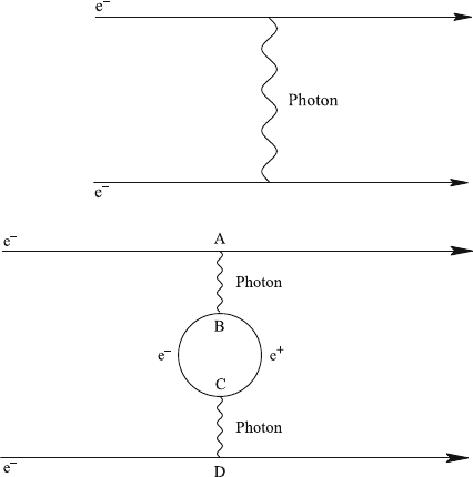
In the case of electron–electron scattering, the simplest diagram is of the form in

Fig.11.1.

With help of the vertices given in Chap.5 we can also draw the diagram in

Fig. 11.2, which is a diagram with four vertices. This diagram describes (amongst

others) the following process: at vertex A an electron emits a photon. At vertex B

this photon decays into an electron–positron pair. After a “loop” this pair annihilates

at vertex C into another photon, which is absorbed by the other electron at vertex D.

We can count the powers of  originating from the vertices, the propagators, and

the remaining factors. Compared to the diagram in Fig. 11.1 with two vertices (where

all powers of  cancel), all diagrams with four vertices contain an additional power

U. Ellwanger, From the Universe to the Elementary Particles, 141

Undergraduate Lecture Notes in Physics, DOI: 10.1007/978-3-642-24375-2_11,

142 11 Quantum Corrections and the Renormalization Group Equations

Fig.11.1 The simplest

diagram contributing to

electron–electron scattering

Fig.11.2 A loop diagram

contributing to

electron–electron scattering

of . An additional power of  means that we are dealing with a quantum effect,

which would vanish in classical electrodynamics obtained in the limit  → 0. For

this reason we denote these contributions as quantum corrections. We should note

that there exist more diagrams with four vertices, which have to be treated in a similar

way as the diagram in Fig. 11.2 in the following.

Next we study the consequences of energy conservation for the energy of each of

the particles; in Fig. 11.2 the photons and the electron–positron pair in the loop are

virtual particles. First we ﬁnd for the electrons in the initial and ﬁnal states, exactly

as in Fig. 11.1 and as discussed in Chap.5, that all their energies are the same if the

momenta before scattering are directed in opposite directions (which we will assume

in the following). It follows that the energies of the virtual photons between A and

B and also C and D vanish.

Concerning the energies of the electron and the positron in the loop, we have to

emphasize that energies of virtual particles can also be negative. Thus energy conser-

vation at the vertices B and C implies that the energies of the electron and the positron

are of the same modulus but of opposite sign, such that their sum vanishes. However,

the moduli of these energies, denoted by Q subsequently, are not determined by

energy conservation!

Which value for Q should we thus chose? The fundamental rule of quantum

mechanics tells us that we have to sum over all the processes that are allowed by

the conservation laws. Hence we have to sum, that is, integrate, over all values of Q

between −∞ and +∞.

Taking the dependence of the propagators of the electron–positron pair on the

energy and hence on Q into account, we ﬁnd that the contribution of the diagram in

11.1 Quantum Corrections 143

Fig. 11.2 to the amplitude contains an integral of the form



∞

+ m

(11.1)

where m

is the electron (and positron) mass, and we have introduced the integration

variable Q

, which is always positive. (In principle we also have to integrate over

the momenta of the electron and the positron; as the ﬁnal result we ﬁnd indeed an

integral of the form (11.1). Actually we would have to replace m

by m

in the

denominator of (11.1); for simplicity we omit these powers of c in the following.)

Let us try to evaluate this integral. First we have to ﬁnd a function F(Q

) whose

derivative with respect to Q

gives the expression under the integral. Up to an irrel-

evant constant, this function is given in our case by

F(Q

) = ln(Q

+ m

). (11.2)

Then the integral (11.1) is obtained by this function with Q

replaced by the upper

limit of the integral less the function evaluated at the lower limit of the integral.

Whereas the evaluation of the function (11.2) at the lower limit Q

= 0ofthe

integral poses no problem (we obtain ln(m

)), we ﬁnd for the function at the upper

limit Q

=∞also +∞, since the logarithm of +∞ is inﬁnite as well – hence no

reasonable result. In the early days of quantum ﬁeld theory this was considered a

serious problem.

Now we treat this problem as follows: instead of integrating over all possible

values of Q

from 0 to +∞, we integrate only over a ﬁnite interval between 0 and

. The quantity Λ

has the following meaning: the expression under the integral

(11.1) was deduced under the assumption that we know the energy dependence of the

propagators (and all other factors contributing to the calculation). However, we can

be sure about this energy dependence only for energies that have been experimentally

veriﬁed. In fact we can assume that the used Feynman rules are valid up to an upper

bound

≤ Λ, but the larger the chosen value of Λ the larger the underlying

assumption. The agreement between high-energy experiments (employing particles

with energiesup to about 1TeV =1000 GeV) and theory(assumingstandard Feynman

rules) allows us to conclude that we can assume Λ  1TeV.

As a result of this reasoning we replace the upper limit of the integral (11.1)by

. Now we obtain a ﬁnite result for this integral, but the result depends on Λ:



+ m

= ln



+ m



 ln





, (11.3)

where we have made the assumption Λ  m

What does this imply for the contribution of the diagram in Fig. 11.2 to the

amplitude of the considered process? Let us compare again the powers of the

coupling constant g , i.e., the ﬁne structure constant α = g

/(4π) of the contribu-

tions of the diagrams in Figs. 11.1 and 11.2 to the amplitude A: the contribution of

the diagram in Fig. 11.1 is of the form α A

(1)

(θ), since it contains two vertices. The

144 11 Quantum Corrections and the Renormalization Group Equations

Fig.11.3 Multi-loop

diagrams contributing to

electron–electron scattering

contributionof thediagram inFig.11.2 is of theformα





(2)

(θ) +...



where we have written explicitly the dependence on Λ, and the dots denote terms

independent of Λ or negligible for Λ  m

. The dependence of A

(1)

(θ) and A

(2)

(θ)

on the momenta of the external electrons can be computed; from (5.28) we obtain,

with (5.21)for



p



, A

(1)

(θ) = 8πm

c/[|p

(1 −cos θ)] since we bracketed off

a factor α.

We explained in Chap.5 that the contributions of the diagrams with four vertices

are relatively small owing to the small value of α. Nowwe see that this conclusion was

not necessarily justiﬁed: if the logarithm multiplying A

(2)

is very large (if Λ  m

holds), the contribution of the diagram in Fig. 11.2 can be even larger than the

contribution of the diagram in Fig. 11.1! (The original conclusion remains valid only

for the terms indicated above by dots, leaving aside the large logarithm.)

In fact (and luckily) we ﬁnd that the dependence of A

(2)

(θ) on the scattering angle

θ, that is, the momenta of the external electrons, coincides with that of A

(1)

(θ) up

to a constant −b. (The negative sign in front of b is a convention.) This allows us to

combine the numerically dominant contributions as follows:

A(θ )  α A

(1)

(θ) +α





(2)

(θ) = α A

(1)

(θ)



1 −b α ln





(11.4)

This is not the end of the story: there exist additional diagrams with more loops

of electron–positron pairs as in Fig. 11.3.

Each loop in a diagram corresponds to another power of α, and implies an addi-

tional power of the logarithm ln





as well as the constant b in the contribution

of the corresponding diagram to the amplitude. We can evaluate the sum over all these

diagrams (a geometric series) and ﬁnd that (11.4) has to be replaced by

A(θ ) =

α A

(1)

(θ)

1 +b α ln





. (11.5)

(We can verify that (11.5) coincides with (11.4) in a power series expansion in α to

the order α

11.2 Energy Dependent Coupling Constants 145

11.2 Energy Dependent Coupling Constants

Now we assume that we want to use electron–electron scattering in order to measure

the ﬁne structure constant α. To this end we proceed as follows: First we measure

the number of scattered electrons as a function of the scattering angle θ,or rather the

probability P(θ). P(θ) is proportional to the square of A(θ ), see (5.29), which allows

us to deduce A(θ ) from the measurement. Finally we compare the result for A(θ )

with the formula

A(θ ) = α

measured

(1)

(θ), (11.6)

where the known expression above for A

(1)

(θ) is used. We emphasize that the

measurement cannot distinguish the contributions of the various diagrams; for this

reason (11.6) is the only reasonable deﬁnition of the measured ﬁne structure constant.

In practice we use processes in atomic physics for the most precise measurements

of α

measured

, but also here we sum automatically over the corresponding Feynman

diagrams.

Comparing the expressions (11.5) and (11.6) we ﬁnd

measured

1 +b α ln





. (11.7)

Accordingly we have to distinguish the “fundamental” coupling constant g

(or rather α = g

/(4π))fromα

measured

! The “fundamental” coupling constant

g is the one connected to the vertices, i.e., the emission or absorption of a photon.

We could measure this fundamental coupling only if we could determine the contri-

bution of the diagram in Fig. 11.1 separately from the contributions of the diagrams

in Figs. 11.2 and 11.3—this is impossible, however, and leads to (11.7)forα

measured

as a function of α and Λ.

We should note that the expression (11.6) contains—by deﬁnition—the measur-

able quantities α

measured

and the θ dependence of A

(1)

but no explicit dependence on

Λ if it is expressed in terms of α

measured

. This is possible since the θ dependence of

the diagrams with loops (denoted as A

(2)

(θ) above) coincides, up to a constant, with

the θ dependence of A

(1)

(θ). A theory in which all relations between measurable

quantities are independent of Λ is denoted as renormalizable: in a renormalizable

theory, Λ can in principle be arbitrarily large (even inﬁnite). (The 1965 Nobel prize

was awarded to S.-I. Tomonaga, J. Schwinger, and R.F. Feynman for, among other

things, the proof that quantum electrodynamics is renormalizable in this sense.) In

Chap.12 we will see that this does not hold for quantum gravity.

Let us return to α

measured

, whose value is known: α

measured

∼ 1/137. This

value was measured in processes at vanishing energies of the photons exchanged in

Figs. 11.1, 11.2, 11.3. We can imagine, however, that α

measured

is measured in a

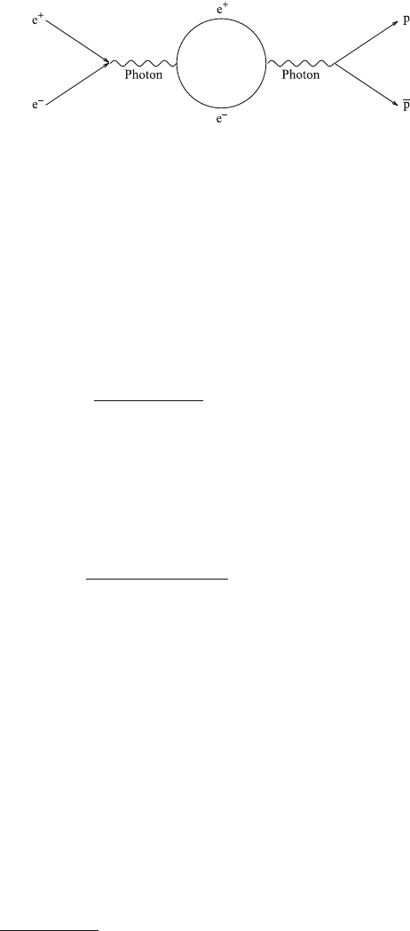
process where the energies of the exchanged photons are no longer small. A typical

example is the pair production of particles p and ¯p described in Chap. 8 in Fig. 8.5.

Here the energy E of the photon is given by E = E(e

) + E(e

−

), which is typically

much larger than the electron mass (multiplied by c

146 11 Quantum Corrections and the Renormalization Group Equations

Fig.11.4 Loop diagram

contributing to

particle–antiparticle

production via

electron–electron

annihilation

Loop diagrams as in Fig.11.2 also contribute to this process, but they are now of

the form of Fig.11.4 and of the rotated Fig. 11.3.

Now we can repeat the previous considerations, starting with the integral over the

energies of the particles e

and e

−

in the loop. In contrast to above, the sum of these

energies no longer vanishes but is equal to the non-vanishing photon energy E,owing

to energy conservation at the vertices. (Still, the difference Q between these energies

is undetermined.) This modiﬁes the propagators of the particles in the loop, and as

a result we ﬁnd that the integral (11.3) over the undetermined energy difference Q

assumes (approximately) the form



+ E

+ m

. (11.8)

All further considerations remain unchanged: as the result for the integral we ﬁnd

the logarithm in (11.3) (with m

replaced by E

+ m

) and the θ dependences of

the amplitudes corresponding to Figs. 8.5 and 11.4 are again the same; hence the

measured ﬁne structure constant α

measured

can again be written as in (11.7)—with

replaced by E

+ m

, however. Then we obtain in the case E

 m

measured

1 +b α ln





. (11.9)

The important consequence of this equation is that, in the case of a measurement

of a ﬁne structure constant at an energy E = 0, the result of the measurement

should depend on the energy! The reason for this energy dependence is the energy

dependence of the contributions of the loop diagrams to the amplitudes.

Apart from the energy E, the following quantities appear in (11.9): the funda-

mental ﬁne structure constant α, the parameter Λ, and the constant b. Whereas the

fundamental ﬁne structure constant α and the parameter Λ are unknown quantities,

the constant b is calculable.

We can show, however, that the energy dependence of α

measured

(we should

write α

measured

(E)) can be given in terms of known quantities only. To this end

we differentiate both sides of (11.9) with respect to ln





(using ln









−ln





) and use (11.9) again on the right-hand side. The result can simply

be written as

dα

measured

(E)

dln





= b α

measured

(E), (11.10)