Ellis A.M., Feher M., Wright T. Electronic and Photoelectron Spectroscopy: Fundamentals and Case Studies

Подождите немного. Документ загружается.

Coupling of angular momenta: electronic states

245

second interaction is very weak and is normally neglected. The ﬁrst interaction is called

spin–orbit coupling. This and the third interaction are invoked to describe the two extreme

cases of coupling in atoms, the Russell–Saunders (also called LS) and the jj schemes.

C.2.1 Russell–Saunders coupling limit

In the Russell–Saunders limit the coupling between the orbital angular momenta is strong.

The source of the coupling is the electrostatic interaction between two electrons. Electron

spins can also couple together, although spin is a magnetic phenomenon and therefore the

coupling is via magnetic ﬁelds, which tends to be a weaker effect than electric ﬁeld coupling.

In Russell–Saunders coupling the interaction between the orbital and spin angular momenta

of a given electron is assumed to be small compared with the coupling between orbital

angular momenta. In this limit the principal torque causes the orbital angular momenta to

precess about a common direction, the axis of the total orbital angular momentum of all

electrons. The spin angular momenta also couple together through the magnetic interaction

of electron spins.

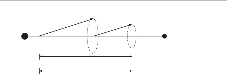
Armed with these assumptions, the vector model described above can be employed to

see the effect of coupling on atoms. For illustration, consider an atom with two electrons

outside its closed shell. The orbital angular momenta of these electrons are represented by

and l

, and the corresponding spin momenta by s

and s

. The coupling of orbital angular

momenta dominates and they form a resultant total orbital angular momentum L = l

+ l

In the same way, the spin momenta also couple to form S = s

+ s

. When this coupling

case is valid, the individual orbital angular momenta l

and l

precess rapidly around L, and

and s

precess rapidly around S. L and S can themselves couple with each other, but this

coupling, known as spin–orbit coupling, is assumed to be relatively weak. As a result, L

and S precess slowly around the resultant total angular momentum J (= L + S).

The signiﬁcance of Russell–Saunders coupling is that a particular electronic state in an

atom is well deﬁned by the quantum numbers L and S. The effect of the weak spin–orbit

coupling results in closely spaced spin–orbit sub-states, designated by the quantum number

J.Asdetailed in Section 4.1, this gives rise to the familiar

2S+1

label for electronic states

in atoms.

C.2.2 jj coupling

The Russell–Saunders scheme describes the electronic states of light atoms rather well but

breaks down for heavier atoms, particularly for the lanthanides and actinides. This is due to

increasing coupling between the orbital and spin angular momenta of individual electrons to

the point where it is no longer negligible, as was assumed in the Russell–Saunders case. In

the limit of very strong coupling between orbital and spin angular momenta, the appropriate

coupling scheme is known as jj coupling. A dominant spin–orbit torque will ﬁrst couple

the spin and orbital momenta of each electron to form resultants, j

= l

+ s

and j

+ s

. The vectors j

and j

interact more weakly, forming the total angular momentum

J = j

+ j

.Injj coupling, l

) and s

) precess rapidly around j

( j

), while j

and

precess slowly around their resultant J.Asaresult, only j

, j

, J and the projection of

246 Appendix C

Ω

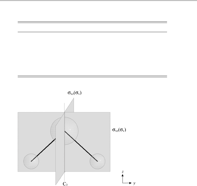
Figure C.2 Illustration of the behaviour of the electronic orbital (L) and spin (S) angular momenta in

a diatomic molecule.

J (M

) are good quantum numbers, i.e. the quantum numbers L and S in the Russell–Saunders

scheme have no signiﬁcance in jj coupling.

Of course it is also possible that the spin–orbit coupling is neither weak enough for

Russell–Saunders to be applicable, nor strong enough for true jj coupling. Description of

this intermediate coupling requires a more mathematical treatment and is not considered

here.

C.3 Coupling of electronic angular momenta in linear molecules

The extension of the above ideas to molecules is not difﬁcult. Consider, for example, a linear

molecule. As in atoms, electrons in this molecule can also possess angular momenta due to

their orbital motion and spin. There is, however, a fundamental difference between atoms and

linear molecules in terms of the environment experienced by electrons. If electron–electron

interactions are neglected, electrons in atoms are subjected to a spherically symmetric ﬁeld,

whereas in a linear molecule a strong axial electric ﬁeld exists between the nuclei and the

interaction with this ﬁeld determines the behaviour of the electrons. This ﬁeld provides a

torque on the orbital motion of the electrons and therefore analogous arguments to those

employed earlier can also be used to construct a vector model of coupled angular momenta

in molecules.

In many-electron molecules, there maybe additional torquesfrom the interaction between

angular momenta. In the most common case, the strongest torque couples the orbital angular

momenta of individual electrons to form a resultant L. Similarly, the spin angular momenta

couple together to form a resultant S.Ifthe spin–orbit coupling is relatively weak, then this

is clearly the molecular analogue of Russell–Saunders coupling in atoms.

The torque exerted by the electrostatic ﬁeld along the molecule is important because

it causes the orbital angular momentum vector to precess around the internuclear axis,

as shown in Figure C.2. This precession is rapid and therefore the corresponding quan-

tum number, L,isnot a good quantum number in this limit. However, the projection of

L along the internuclear axis, denoted by the symbol ,isaconstant of motion and is

therefore a good quantum number. To determine the possible values of , the contribu-

tions from individual electrons must be considered. With only one unpaired electron, the

Coupling of angular momenta: electronic states

247

total orbital angular momentum is the orbital angular momentum of that sole electron, and

we can identify a corresponding one-electron orbital angular momentum quantum num-

ber λ = 0, 1, 2, 3, etc., which corresponds to σ, π, δ, and φ orbitals, respectively (see

Section 4.2.2). Note that the orbitals with non-zero λ are doubly degenerate, which may

be viewed as being due to the two possible directions for rotation of the electrons around

the internuclear axis, clockwise or anticlockwise. In this sense the projection of orbital

angular momentum on the internuclear axis is a signed quantity, but the convention is that

λ is always quoted as a positive number. The reader should recognize however that if,

for example, λ = 1 then the actual orbital angular momentum along the internuclear axis

is +

h or −h.

If there is more than one electron, each electron will contribute ±λ

h to the orbital

angular momentum along the internuclear axis. All ﬁlled orbitals will therefore make a

zero contribution to  since the orbital angular momenta of the electrons in these orbitals

cancel. If there are two unpaired electrons, say one in a π orbital and one in a δ orbital, the

possible angular momenta are ±

h, ±2 h, or ±3 h. These correspond to  = 1, 2, or 3 and

the resulting electronic states are labelled as , , and  electronic states, respectively. A

better and more general way of deriving the possible orbital angular momentum states is

by recognizing that the σ, π, δ, etc., labels are actually symmetry labels for the molecular

orbitals, i.e. they are irreducible representations of the appropriate linear molecule point

group, D

∞h

or C

∞v

. The overall angular momentum must therefore also correspond to one

of the irreducible representations of the point group and can be obtained by taking the

direct product of the symmetries for each occupied orbital, and taking appropriate care in

the application of the Pauli principle (see below). This was the recommended procedure

covered in Part I.

The axial electric ﬁeld in linear molecules does not have a direct effect on the spin angular

momenta, since spin is a magnetic phenomenon. However, when  = 0 the orbiting motion

of the electron(s) generates a magnetic ﬁeld,

which can also cause the total spin angular

momentum, S,toprecess around the internuclear axis. This is none other than spin–orbit

coupling, but if the spin–orbit coupling is not as strong as the spin–spin coupling then S

remains a good quantum number. As in the case of orbital angular momenta, the projection

of S onto the internuclear axis is quantized. The projection quantum number is given the

symbol ,which is unfortunately the same as the label used to designate electronic states

with  = 0. The allowed values of  are −S, −S + 1,...,+S,where S may be integer or

half integer depending on the number of unpaired electrons.

As in the case of atoms, spin–orbit coupling leads to spin–orbit sub-states with different

energies. In this case the total electronic (orbital + spin) angular momentum is given by

the quantum number  (=  + ). Although  is, like , ostensibly a signed quantum

number, the accepted convention is to quote the positive value, i.e.  =| + |. The

complete label for electronic states in linear molecules is then

2S+1





As an example, consider the case of two electrons in two different π molecular orbitals

(the choice of different π orbitals avoids difﬁculties with the Pauli exclusion principle – see

Current ﬂowing in a circular conductor generates a magnetic ﬁeld perpendicular to the plane of the conductor.

We can use the same analogy for an orbiting electron around the internuclear axis to explain how it generates a

magnetic ﬁeld due to its orbital motion.

248 Appendix C

Appendix E). As λ = 1 for a π-electron,  can be 2 or 0, i.e.  or  electronic states are

possible. The  state is doubly degenerate but there are two different  states, a 

and

a 

−

due to the ﬁner interactions of the electrons (a ﬁnding that is best seen by evaluating

the direct product π ⊗ π). The net spin S for the two electrons is 0 or 1, giving rise to

the multiplicities 1 and 3. The possible electronic states that may result from the π

1

conﬁguration are therefore



−



−

 and

.

C.4 Non-linear molecules

The presence of off-axis nuclei in non-linear molecules usually results in all electronic

orbital angular momentum being quenched. The only exceptions to this are high symmetry

molecules in spatially degenerate electronic states. A good example is benzene, which in

its ground electronic state has the outer electronic conﬁguration...(1a

)

(1e

)

. The

resulting electronic state is a

state, in which there is no net orbital or spin angular

momentum. If, however, an electron is removed from the HOMO, the resulting ground state

of the cation is a

state. E

is a doubly degenerate representation and so the ground

electronic state of the cation does possess orbital angular momentum. The source of this

orbital angular momentum is the unimpeded circulation of the unpaired electron in the π

system above and below the nuclei in the benzene ring. In the ground state of benzene the net

orbital angular momentum is zero because all orbitals are full and therefore the clockwise

and counterclockwise contributions cancel. However, in the benzene cation this is no longer

the case and spin–orbit coupling splits the resulting

state into two spin–orbit sub-states,

which are labelled

1g(1/2)

and

1g(3/2)

Although orbital angular momentum can exist in non-linear molecules with degenerate

electronic states, it is important to recognize that it will still be quenched to a greater or lesser

extent. For example in the benzene cation the Jahn–Teller effect, which couples electronic

orbital and vibrational motions, acts to quench some of the pure orbital angular momentum.

Further reading

Molecular Quantum Mechanics, 3rd edn., P. W. Atkins and R. S. Friedman, Oxford, Oxford

University Press, 1999.

Angular Momentum,R.N.Zare, New York, Wiley, 1988.

Angular Momentum in Quantum Mechanics,A.R.Edmonds, Princeton, Princeton

University Press, 1996.

Appendix D

The principles of point group

symmetry and group theory

Molecular symmetry is of great importance in the discussion of spectroscopy. It helps

to simplify the explanation of complex phenomena, such as molecular vibrations, and

is an important aid in the derivation of electronic states and transition selection rules.

It also simpliﬁes the application of molecular orbital theory, which is often applied to

assign or predict electronic spectra. In many cases, it provides strikingly simple answers to

complicated questions.

In its original form, group theory is a rigorous mathematical subject. No attempt will

be made here to be rigorous – the aim is simply to summarize the basics as they apply

to symmetry, in light of which the spectroscopic applications of the theory can become

clearer. Although the concepts introduced here might be valid for any object with symmetry

elements, we will apply these only to molecules. This appendix is not intended to be a

comprehensive account of point group symmetry and group theory. Instead the intention is

to review some of the key principles required for applications in electronic spectroscopy.

Anewcomer to the subject of symmetry and group theory is ﬁrst advised to consult an

appropriate textbook on this topic, such as one of those listed in the Further Reading at the

end of this appendix.

D.1 Symmetry elements and operations

We begin with two fundamental concepts, symmetry operations and symmetry elements.

Symmetry operations are transformations that move the molecule such that it is indistin-

guishable from its initial position and orientation. For example, the water molecule has

mirror image symmetry. An imaginary mirror perpendicular to the molecular plane and

passing through the oxygen atom will interchange the two hydrogen atoms, leaving the

molecule unchanged in its appearance. This reﬂection operation is an example of a sym-

metry operation and is denoted by the symbol σ .

Symmetry elements are geometric objects, such as points, lines or planes. For water, the

symmetry element considered so far is a plane of reﬂection. The water molecule has another

mirror plane, this second one being in the plane of the molecule. The two corresponding

249

250 Appendix D

Table D.1 Symmetry elements and symmetry operations

Symmetry element Symmetry operation Symbol

Identity operation (does nothing) E

Plane Reﬂection through a plane σ

Axis Rotation 360

◦

/n around an n-fold axis C

Centre of symmetry (or

inversion)

Inversion through a point i

Improper axis (rotation axis

and a perpendicular

plane)

Rotation 360

◦

/n about an axis followed

by reﬂection through a plane

perpendicular to the axis

Figure D.1 Symmetry elements of the water molecule.

symmetry operations are distinguished by their subscripts, referring to the chosen coordinate

system, as shown in Figure D.1.Inaddition to mirror planes, the water molecule has a two-

fold axis of rotational symmetry that bisects the HOH angle: rotation of the molecule around

this axis by 180

◦

leaves the molecule unchanged.

There are ﬁve types of symmetry operations that are used for molecules and the corre-

sponding symmetry elements are summarized in Table D.1.

As can be seen from the ﬁnal column of Table D.1, the symbols used to denote symmetry

operations are often accompanied by a subscript. For example, to express that the rotation

of the object by 360

◦

/n leaves it indistinguishable, the applied operation is denoted as

, e.g. the 180

◦

rotational symmetry of H

Oisdenoted as C

. Another symmetry operation

in which rotation plays a part is improper rotation.For example, S

expresses a six-fold

improper rotation that consists of a 60

◦

rotation (360

◦

/6) about an axis followed by reﬂection

in the plane perpendicular to the axis.

The principles of point group symmetry and group theory

251

Planes of reﬂection are labelled to indicate their relative orientation in the coordinate

system. The reﬂection in the plane that includes the principal axis of rotation (the axis

of highest rotational symmetry) is said to be vertical and is labelled as σ

. Mirror planes

perpendicular to this are referred to as horizontal and are denoted by σ

.Insome cases

when there is more than one symmetry plane of the same kind (such as the two σ

planes of

water shown in Figure D.1), they are distinguished by subscripts showing which plane they

include (e.g. σ

and σ

). If an operation is to be performed several times, this is shown as

a superscript, e.g. C

signiﬁes that the C

operation is to be carried out twice such that a

rotation of 240

◦

takes place.

The identity operation, E,israther odd in that it corresponds to no net movement of any

atom in the molecule. However, this operation is always included because it is important in

the mathematics of group theory, as will be seen later. Some operations are equivalent to

E. Examples of this are C

(indicating a 360

◦

rotation), i

and σ

. Improper rotations are

less straightforward: S

implies n rotations and n reﬂections in the plane and this can lead

to identity only if n is even.

D.2 Point groups

The collection of symmetry operations applying to molecules of a particular symmetry is

called a point group. There are a number of different point groups and the properties of these

are collected in character tables. Determining which point group the molecule belongs to

is the ﬁrst step in utilizing molecular symmetry.

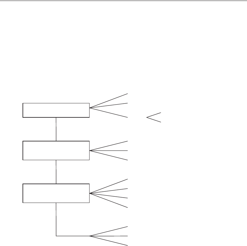
The diagram below helps in the identiﬁcation of the most commonly occurring point

groups. The classiﬁcation is achieved by answering a series of simple questions. The ﬁrst

question relates to special groups. These include the two groups for linear molecules,

∞h

and C

∞v

. These point groups are distinguished by whether or not they have a centre of

symmetry (operation i in the above table). Thus, for example, CO

has a centre of symmetry

(positioned at the carbon atom) and therefore belongs to the D

∞h

point group. In contrast,

CO does not possess a centre of symmetry and so has C

∞v

point group symmetry. Other

special groups include tetrahedral (T

, e.g. the CH

molecule), octahedral (O

, e.g. SF

and icosohedral (I

, e.g. C

If a molecule does not belong to any of these special groups, then a series of rules can

be used to establish its point group. The starting point is to determine the principal axis

of rotation. In the ﬂow chart below, the letter n in the name of the point groups indicates

the order of the principal axis. If there is no such axis (other than C

,which is equivalent

to E), there might only be a symmetry plane (this is the case in the C

group), or an inversion

centre (in the C

group). Molecules with no symmetry other than identity belong to the

group.

If the molecule has an n-fold principal axis, further classiﬁcation depends on whether

or not this is only the consequence of a 2n-fold improper axis (if the answer is yes

the point group is designated as S

). Molecules belonging to the S

point groups are

rare.

252 Appendix D

The remaining groups are denoted with the letters C or D. The former have no C

axis

perpendicular to the principal axis, whereas the latter have such axes. If a σ

plane exists

(i.e. a plane perpendicular to the principal axis), the group is labelled C

or D

. Molecules

in the C

and D

groups have no σ

plane, only one or more σ

planes, i.e. containing

the principal axis. Here the d subscript arises because the axes of rotational symmetry

perpendicular to the principal one do not contain the σ

planes; these planes dissect the

angle between the axes. Such planes are referred to as dihedral and marked as σ

.Ifthere

is no σ

plane, the point group is called C

or D

Is it a special group?

Is there a rotation (C

) axis

of order n ≥ 2?

Is there more than one C

axis with n

≥

Octahedral, O

Tetrahedral, T

Linear

∞

(if i symmetry element is missing)

∞

(if i symmetry element exists)

(if no other symmetry element exists)

(if it also has one

plane)

(if it has n

planes)

(if it has an S

axis coaxial with the principal axis)

(if no other symmetry element exists)

(if only one reflection plane exists)

(if only a centre of inversion exists)

(if no further symmetry elements exist)

(if it has n

planes bisecting the C

axes)

(if it also has one

plane)

D.3 Classes and multiplication tables

Afew properties of point groups are described below, which can be derived from the general

properties of mathematical groups.

Point groups can be characterized by the different applicable symmetry operations

possible within the group.

Multiplication is the subsequent execution of two symmetry operations. The multipli-

cation of symmetry operations is associative (e.g. (AB)C = A(BC)) but not necessarily

commutative (e.g. AB = BA is possible).

Each symmetry operation has an inverse, such that the operation multiplied with its

inverse gives the identity operation.

The principles of point group symmetry and group theory

253

Table D.2 Multiplication table for symmetry

operations of the C

point group







E EC







E σ



























Table D.3 Similarity transformations for C

point group

Similarity transformation EC







EXE

−1







)

−1







)

−1







(σ

)

−1

Xσ







(σ

)

−1

Xσ







(σ

)

−1

Xσ







Point groups must contain the products of all pairs of elements, the squares of all

elements and the reciprocals of all elements.

The total number of elements is called the order of the group.

These concepts will be demonstrated for the C

point group. A molecule with this point

group symmetry is NH

.Ithas the following symmetry elements: E (identity operation),

(120

◦

rotation about a three-fold axis), C

(240

◦

rotation about a three-fold axis), σ





, and σ



(reﬂection through one of the three equivalent mirror planes, each containing

an N

H bond in the case of NH

). The multiplication table for the point group is shown

in Table D.2 (where the column and row heading show the symmetry operations that are

multiplied).

The symmetry operations of the point group can be subdivided into classes. If A, B, and

X are elements of a group, then the operation XAX

−1

is called a similarity transformation.

If the relationship XAX

−1

= B holds, A and B are said to be conjugates. A class consists of

a complete set of elements that are conjugates of each other.

Looking at the multiplication table of the C

group, it can be established that the three

operations belong to the same class, as do C

and C

, because they are connected by

similarity transformations (see Table D.3). The identity operation is in a class of its own.

In general the E, i and σ

operations are always in a class of their own. In contrast, all σ

operations of a group form a class together, as do the σ

operations.

254 Appendix D

D.4 The matrix representation of symmetry operations

All symmetry operations correspond to geometrical transformations and can be repre-

sented by matrices. Each such matrix represents a single operation. These matrices obey

the same multiplication rules as the symmetry operations. The effect of different sym-

metry operations on an arbitrary point, represented by its coordinates (x, y, z), will be

shown for the water molecule. This will be done by using the matrix representation of the

operations.

In the C

point group for the water molecule, the identity operation can be represented

byaunit matrix:





100

010

001





















(D.1)

Notice that the coordinates of the arbitrary point are expressed as a column matrix.

According to the axis scheme shown in Figure D.1, the C

operation reverses the sign of

the x and y coordinates and so is equivalent to the 3×3 matrix shown below:





−100

0 −10

001

















−x

−y





(D.2)

Reﬂection through the xz plane reverses the sign of the y coordinate and in matrix notation

is equivalent to





100

0 −10

001

















−y





(D.3)

The matrix representations are often complicated to deduce. Luckily, as will be seen later,

for practical purposes it is unnecessary to derive these representations. It should be noted

that these matrices are 3×3 because they were derived for a triatomic molecule. The dimen-

sionality of these transformation matrices depends on the number of atoms in the system.

The actual composition of the matrices is also determined by the choice of coordinate

system. Hence in any point group, it is possible to devise an inﬁnite number of matrix

representations of the symmetry operations.

If a similarity transformation exists that transforms all matrices of the representation

into block diagonal form, the initial representation is said to be reducible.Ablock-diagonal

matrix has the appearance of a matrix constructed from smaller matrices located along

the diagonal. Such a matrix can be illustrated by the following 9×9 matrix that has been