Ellis A.M., Feher M., Wright T. Electronic and Photoelectron Spectroscopy: Fundamentals and Case Studies
Подождите немного. Документ загружается.


23 Vibrationally resolved spectroscopy of complexes
195
Table 23.3 Dissociation energies (D
0
in cm
−1
)
for Mg
+
–Rg complexes
Complex X
2
+
A
2
Mg
+
–Ne 110 1700
Mg
+
–Ar 1280 5550
Mg
+
–Kr 1920 7130
Mg
+
–Xe 4180 11030
The anharmonicities progressively decrease as the rare gas group is descended. This
is because, as the bond strengthens, the potential well becomes more harmonic-like
(i.e. parabolic) for the vibrational energies sampled in the photodissociation experiment.
23.7 Dissociation energies
The extensive vibrational progressions can be used to estimate the dissociation energies of
the Mg
+
–Rg in their A
2
electronic states. The dissociation energy, D
0
,issimply the sum
of the separations between all the vibrational energy levels, starting from v
= 0, i.e.
D
0
=
v
G
v
+
1
/
2
(23.4)
where
G
v
+
1
/
2
= G(v
+ 1) − G(v
) (23.5)
are vibrational term values (see Section 5.1.2). If the positions of most of the bound energy
levels have been measured from the spectrum, then the area under a plot of G
v
+
1
/
2
versus
v
+
1
2
extrapolated to G
v
+
1
/
2
= 0 will give an accurate dissociation energy.
In practice the vibrational structure observed in an electronic spectrum represents only
a modest subset of the total set of vibrational energy levels. In this case the Birge–Sponer
extrapolation can be employed. This extrapolation is based on the assumption that the
potential energy curve is adequately described by a Morse potential, i.e. the anharmonicity
constant x
e
is sufficient to account for all of the anharmonicity and the vibrational term
value G(v)isaccurately described by equation (5.14). With this approximation it is easy to
show that
G
v
+
1
/
2
= ω
e
− 2ω
e
x
e
(v
+ 1) (23.6)
and therefore a plot of G
v
+
1
/
2
versus v
should be linear and can readily be extrapolated
to G
v
+
1
/
2
= 0, allowing D
0
to be estimated.
Table 23.3 shows the dissociation energies obtained. Notice that dissociation energies
for the ground electronic states are also included in the table. These can be determined from
the expression
D
0
= D
0
+ v
00
− E(
2
P−
2
S) (23.7)

196 Case Studies
which follows from the conservation of energy. The quantity ν
00
is the A
2
v
=
0 ← X
2
+
v
= 0 electronic transition energy and E(
2
P−
2
S) is the energy required
to excite the unpaired electron in the free Mg
+
ion from the 3s to the 3p orbital.
The dissociation energies show the trends expected from the earlier discussion about
electronic structures. Each complex is much more strongly bound in its A
2
state than
in the X
2
+
state due to the reduced shielding of the positive charge when the unpaired
electron density has a π orientation. Furthermore, there is a dramatic increase in binding
energy for both electronic states in moving progressively from Ne to Xe due to the increasing
polarizability of the rare gas atom.
23.8 B–X system
In the Mg
+
–Ne photodissociation spectrum in Figure 23.2 there is a prominent broad
feature in addition to the sharp bands discussed above. Duncan et al. attribute this to the
B
2
+
−X
2
+
electronic transition. The binding energy of the B
2
+
state is likely to be
even less than that of the X
2
+
state because of the increased electron–electron repulsion
between Mg
+
and the Ne atom, a result of the orientation of the 3p
z
orbital along the
internuclear axis. There will therefore be very few if any bound vibrational levels and
the separation between them will be exceedingly small, explaining why there is no evidence
of any resolvable vibrational structure. In fact most of the band envelope is likely to arise
from excitation to the continuum of states above the dissociation limit of the B
2
+
state.
References
1. J. S. Pilgrim, C. S. Yeh, K. R. Berry, and M. A. Duncan, J. Chem. Phys. 100 (1994) 7945.
2. J. E. Reddic and M. A. Duncan, J. Chem. Phys. 110 (1999) 9948.

24
Rotationally resolved
spectroscopy of Mg
+
–rare
gas complexes
Concepts illustrated: ion–molecule complexes; photodissociation spectroscopy; Hund’s
coupling cases; rotational structure in open-shell molecules; least-squares fitting of
spectra.
This Case Study follows on from the previous one. However, rotationally resolved pho-
todissociation spectra are the focus here, specifically for Mg
+
–Ne and Mg
+
–Ar. Although
these ions are diatomic species, their rotationally resolved spectra are not trivial to
analyse. The reason for this is the presence of an unpaired electron, which gives rise to
a net spin angular momentum which can interact with the overall rotation of the complex
(spin–rotation coupling). In addition, in some electronic states there may also be a net orbital
angular momentum, and this can interact both directly with the molecular rotation (giving
rise to the phenomenon known as doubling) and with the electron spin. The latter is much
the strongest of these angular momentum interactions and its effect can be readily seen in
the rotationally resolved spectra, as will be discussed below.
Duncan and co-workers have recorded partly rotationally resolved electronic spectra
for the A
2
−X
2
+
transitions of Mg
+
–Ne and Mg
+
–Ar, and these form the basis of the
Case Study described here [1, 2]. A photodissociation technique was employed as detailed
in Chapter 23. Before describing the spectra and their analysis, the expected rotational
energy level structure for the X
2
+
and A
2
electronic states is considered. Much of this
description is similar to that met for NO in Chapter 22.
24.1 X
2
Σ
+
state
Figure23.1 in the previous Case Study provides a simple and extremely useful representation
of the electronic structure of Mg
+
–Rg cations in their two lowest electronic states. The
electrons on the rare gas atom are in tightly bound orbitals and require very high energies to
excite to vacant orbitals. The remaining electrons are strongly localized on Mg
+
, and all but
one occupy core orbitals. Consequently, the lowest-lying electronic states in Mg
+
–Rg are
197
198 Case Studies
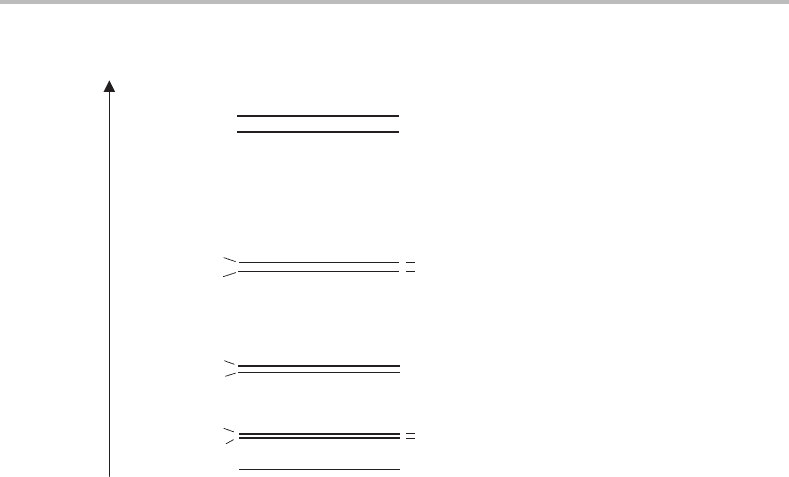
0
Energy
1/2
1/2
3/2
3/2
5/2
5/2
7/2
7/2
9/2
J
1
2
3
4
N
+
+
+
+
+
Figure 24.1 Rotational energy levels of a diatomic molecule in a
2
+
electronic state satisfying
Hund’s case (b) coupling. The total angular momentum quantum number J is given by J = N ±
1
/
2
,
where N is the rotational quantum number. The + or − beside each energy level refers to the parity
(see text).
differentiated by the orbital occupied by the unpaired electron, and in the ground electronic
state this can be described approximately as the Mg
+
3s orbital. The resulting electronic
state in the complex is a
2
+
state.
The unpaired electron in this state has a non-zero spin angular momentum, which can
interact with the angular momentum generated by overall rotation of the molecule. Inter-
action must proceed via magnetic coupling, since electron spin is a purely magnetic effect.
The rotation of Mg
+
–Rg will generate oscillating electric and magnetic fields and the latter
can directly couple with the electron spin. However, it is important to note that indirect
magnetic coupling is also possible via orbital motion of the electrons and so even in open-
shell homonuclear diatomic molecules a spin–rotation interaction can occur. Regardless of
the mechanism, in almost all cases spin–rotation coupling is very weak.
The coupling between spin and rotational motion in Mg
+
–Rg is an example of Hund’s
case (b) coupling. The basic principles of Hund’s coupling cases are outlined in Appendix
G and were also met in Chapter 22. The total angular momentum quantum number for
the molecule, J,isgivenbyJ = N ±
1
/
2
,where N is the rotational quantum number
(= 0, 1, 2, 3, etc.). The two possible values of J,which arise for all rotational levels except
for N = 0, are due to the two possible orientations of the electron spin (up or down). Con-
sequently, each rotational level is actually split into two levels when spin–rotation coupling
occurs, as shown in Figure 24.1. The magnitude of the splitting increases with the speed
of rotation, and is given by γ (N +
1
/
2
)where γ is a quantity known as the spin–rotation

24 Rotationally resolved spectroscopy of complexes
199
coupling constant. In most molecules the effect of spin–rotation coupling is very small and
can only be resolved using high resolution spectroscopy.
24.2 A
2
Π state
The first excited electronic state in Mg
+
–Rg corresponds to an electron excited to the 3pπ
orbitals. These orbitals form a degenerate pair and as a result the unpaired electron can
orbit unimpeded around the internuclear axis with an orbital angular momentum given
by the quantum number λ = 1. In the resulting
2
electronic state, the strongest angular
momentum interaction occurs between the orbital and spin angular momenta of the unpaired
electron. This spin–orbit coupling in Mg
+
–Rg was discussed in some detail in the previous
Case Study. If the spin–orbit coupling constant, A, has a magnitude such that A BJ, then
Hund’s case (a) coupling applies.
1
In the Hund’s case (a) limit the torque provided by the
electrostatic field of the nuclei locks the orbital angular momentum into precessional motion
about the internuclear axis. This precession generates a concomitant magnetic field, which
in turn forces the spin angular momentum to precess sympathetically about the internuclear
axis. The quantum numbers describing this coupled electronic motion are , S, , and .
and are the quantum numbers describing the projection of orbital and spin angular
momenta along the internuclear axis.
2
For Mg
+
–Rg the values are = 1 and =
1
2
. is
the vector sum of | + | and may take on the values of
1
2
and
3
2
in this specific example.
S is a good quantum number in both Hund’s cases (a) and (b).
Spin–orbit coupling splits the
2
electronic state into two spin–orbit components,
2
1/2
and
2
3/2
,where the subscript refers to the value of . Each of these sub-states has its
own set of rotational levels, as shown in Figure 24.2. The rotational levels are distinguished
by their total angular momentum quantum number, J, and the identity of the particular
spin–orbit sub-state. One can identify a rotational quantum number with values R = 0,
1, 2, 3, etc., such that J = R + . Thus in the
2
1/2
state the smallest possible value
of J is
1
2
whereas in the
2
3/2
state it is
3
2
. This has consequences for the spectra, which
will be seen later.
Additional labels, + and −, are included for the rotational levels in both Figures 24.1
and 24.2. These refer to the parity of the energy level. Parity is a symmetry label, but one
that results from the operation in which the coordinates of all particles in the molecule
(nuclei and electrons) are inverted with respect to a space-fixed coordinate system. This is
an involved concept and will not be developed in any detail here; sophisticated treatments
can be found in many books (see for example References [3] and [4]). Parity is a useful
description of symmetry that aids in establishing transition selection rules, as detailed below.
1
In fact, when the spin–orbit coupling is strong there are two possible coupling cases, Hund’s cases (a) and (c). See
Appendix G for more details.
2
Note the potential for confusion here. As well as its use to designate electronic states in linear molecules with
orbital angular momentum = 0, the symbol is unfortunately also used to designate the quantum number for
projection of the electronic spin angular momentum on the internuclear axis.

200 Case Studies
1/2
3/2
5/2
7/2
9/2
J
+
+
+
+
+
3/2
5/2
7/2
9/2
J
+
+
+
+
2
Π
1/2
2
Π
3/2
Figure 24.2 Rotational energy levels of a diatomic molecule in a
2
electronic state satisfying Hund’s
case (a) coupling. Two sets of levels are shown corresponding to the spin–orbit components
2
1/2
and
2
3/2
. The overall angular momentum quantum number is given by the half integer quantum number
J. The + or − beside each energy level refers to the parity (see text).
24.3 Transition energies and selection rules
The transitions must satisfy the usual single-photon selection rule for the overall angular
momentum, J =0, ±1. In addition, there is a selection rule based on parity, which derives
from the fact that the dipole moment operator, µ,isalinear function of the positions of
all the particles in the molecule (see equation (7.2)). Application of the parity operation
switches the coordinates of the particles to their negative values and since this makes µ
change sign the dipole moment operator must possess negative parity. For an electric dipole
driven transition the transition moment is given by the integral expression in equation (7.1),
and this will be zero if the integrand has negative parity. If the parity in upper and lower
states is the same, for example both are positive, then the parity of the integrand is
(+) ⊗ (−) ⊗ (+) = (−). Consequently, in an electric-dipole allowed transition the par-
ity must change between the upper and lower states.
Armed with the above selection rules, it is possible to identify the allowed transitions, and
these are shown in Figure 24.3. The rotational structure is more complicated than a simple
three-branch P/Q/R structure. Focussing on the
2
1/2
−
2
+
sub-band, six branches can be
identified. These can be divided into P, Q, and R branches but additional subscripts are
added to the labels to designate the specific upper and lower levels. Such ideas were met in
24 Rotationally resolved spectroscopy of complexes
201
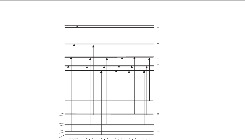
1/2
1/2
3/2
3/2
5/2
5/2
7/2
7/2
9/2
1/2
3/2
5/2
7/2
9/2
J
+
+
2
Π
1/2
+
+
+
+
+
+
+
+
+
2
Σ
+
R
11
R
12
Q
11
Q
12
P
11
P
12
Figure 24.3 Allowed transitions in a
2
1/2
−
2
+
electronic absorption band. Six branches occur, as
shown at the bottom of the diagram. If the spin–rotation coupling in the
2
+
state is too small to
be resolved then the R
12
and Q
11
transitions are indistinguishable, as are the Q
12
and P
11
transitions,
reducing the number of observable branches to four.
Case Study in Chapter 22, and the interested reader can also find out more by consulting the
textbook by Herzberg [5]. The important thing to note is that if the spin–rotation splitting is
too small to be resolved then the number of distinguishable branches is reduced to four. In
those cases where the rotational constant is similar in the upper and lower electronic states,
the branches have a structure where the spacing between adjacent transitions is roughly 3B,
B, B, and 3B (moving from low energy to high energy). These spacings correspond to the
P
12
, P
11
+ Q
12
, Q
11
+ R
12
, and R
11
branches, respectively.
24.4 Photodissociation spectra of Mg
+
–Ne and Mg
+
–Ar
Figures 24.4 and 24.5 show rotationally resolved photodissociation spectra of Mg
+
–Ne and
Mg
+
–Ar. In neither spectrum is the zero-point vibrational level accessed in the A
2
state.
This is because the Franck–Condon factors for 0–0 transitions are small for these ions, and
adequate signal-to-noise ratios were only obtained for rotational structure in transitions to
higher vibrational levels.
The spectrum for Mg
+
–Ne looks to be quite simple, but its appearance is deceptive;
the limited spectral resolution means that many peaks are actually superpositions of two
or more transitions. From Chapter 23 we know that the complex will be far more strongly
bound in the excited electronic state than in the ground state. The rotational constant in the
A
2
state should therefore be substantially larger than that in the X
2
+
state. The marked
change in rotational constants will give rise to band head formation (see also Chapter 16)

202 Case Studies
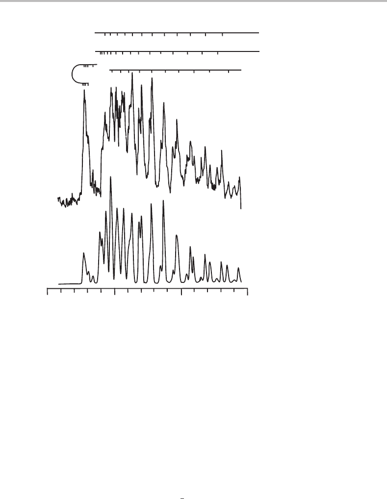
35368 35373 3537835363
Wavenumber/cm
−1
Mg
+
photofragment intensity
Figure 24.4 Rotationally resolved photodissociation spectrum of Mg
+
–Ne. The features shown have
been assigned to the A
2
1/2
−X
2
+
9–0 band by Reddic and Duncan [1]. The upper trace shows
the experimental spectrum while the lower trace is a simulation based on an assumed rotational
temperature of 4 K. (Reproduced with permission from J. E. Reddic and M. A. Duncan, J. Chem.
Phys. 110 (1999) 9948, American Institute of Physics.)
in some branches and rapidly divergent rotational structure in other branches. This is exactly
the structure seen in Figure 24.4.Itturns out that the spectrum in Figure 24.4 is due to the
A
2
1/2
−X
2
+
transition rather than the A
2
3/2
−X
2
+
electronic transition, as justified
later. The lowest energy feature in the spectrum is the P
12
branch, which is relatively weak.
The remaining, and much stronger features are due to the P
11
+ Q
12
, Q
11
+ R
12
, and R
11
branches and all of the strong peaks contain unresolved contributions from at least two of
these branches.
With so much unresolved structure it would be impossible to extract precise rotational
constants from the spectrum in Figure 24.4.Itisevenarather difficult task to assign the peaks
to specific rotational transitions without the aid of computer simulation, but with simulations
important information can be extracted readily from the spectrum. Reddic and Duncan used
a program known as SpecSim to simulate the rotational structure in a
2
−
2
+
spectrum.
An outline of how this and similar programs work is given in Appendix H. Most of these
programs are equipped with the option of varying spectroscopic constants in a systematic
(least-squares) fashion such that the best possible agreement (the best fit) between theory
and experiment is obtained.
Rotational constants of 0.343 ± 0.013 and 0.238 ± 0.008 cm
−1
were extracted for the
upper and lower states of Mg
+
–Ne. These can be used to estimate bond lengths of 2.59 ±
0.05 Å and 3.17 ± 0.05 Å, respectively. The spectrum in Figure 24.4 involves the v = 9
vibrational level in the A
2
state, and the larger amplitude of the vibrations in this highly
excited level will yield a larger effective bond length than would be the case in the v = 0
24 Rotationally resolved spectroscopy of complexes
203
32786 32791 32796
32801
Wavenumber/cm
−1
P
22
(J )
2.5
9.5
9.58.57.56.55.5
R
21
(J)
Q
22
(J) + P
21
(J + 1)
Q
21
(J + 1) + R
22
(J)
15.514.513.512.511.510.5
11.510.59.58.57.56.55.5
Figure 24.5 Rotationally resolved photodissociation spectrum of Mg
+
–Ar. The features shown have
been assigned to the A
2
3/2
−X
2
+
5–0 band by Scurlock and co-workers [2]. The upper trace
shows the experimental spectrum while the lower trace is a simulation based on an assumed rotational
temperature of 4 K. (Reproduced with permission from C. T. Scurlock, J. S. Pilgrim, and M. A.
Duncan, J. Chem. Phys. 103 (1995) 3293, American Institute of Physics.)
level. Nevertheless, it is clear that much shorter bond lengths are obtained in the A
2
state
and this is consistent with the expected stronger binding in this state compared with the
X
2
+
state.
The findings are similar for the Mg
+
–Ar spectrum in Figure 24.5. Note that here the
simulations show that the band is due to the A
2
3/2
−X
2
+
transition. The best way to
distinguish between the
2
3/2
−
2
+
and
2
1/2
−
2
+
transitions is by noting that certain
transitions present in the latter are missing in the former because the lowest possible value
of J in the
2
3/2
component is J =
3
2
. Simulations, or if the resolution is sufficient even
simple inspection, should allow an assignment to
2
3/2
−
2
+
or
2
1/2
−
2
+
transitions.
A least-squares fit of the rotational structure allowed bond lengths of 2.882 ± 0.017 Å
and 2.524 ± 0.014 Å to be deduced for the X
2
+
and A
2
states of Mg
+
–Ar. As with
Mg
+
–Ne, there is a marked shortening in bond length upon electronic excitation due to the
much stronger binding in the excited electronic state.

204 Case Studies
References
1. J. E. Reddic and M. A. Duncan, J. Chem. Phys. 110 (1999) 9948.
2. C. T. Scurlock, J. S. Pilgrim, and M. A. Duncan, J. Chem. Phys. 103 (1995) 3293.
3. Molecular Symmetry and Spectroscopy,P.R.Bunker and P. Jensen, Ottawa, NRC Research
Press, 1998.
4. Angular Momentum: Understanding Spatial Aspects in Chemistry and Physics,R.N.Zare,
New York, Wiley, 1988.
5. Molecular Spectra and Molecular Structure. I. Spectra of Diatomic Molecules,G.Herzberg,
Malabar, Florida, Krieger Publishing, 1989.