Dougherty С. Introduction to Econometrics, 3Ed

Подождите немного. Документ загружается.

TRANSFORMATIONS OF VARIABLES

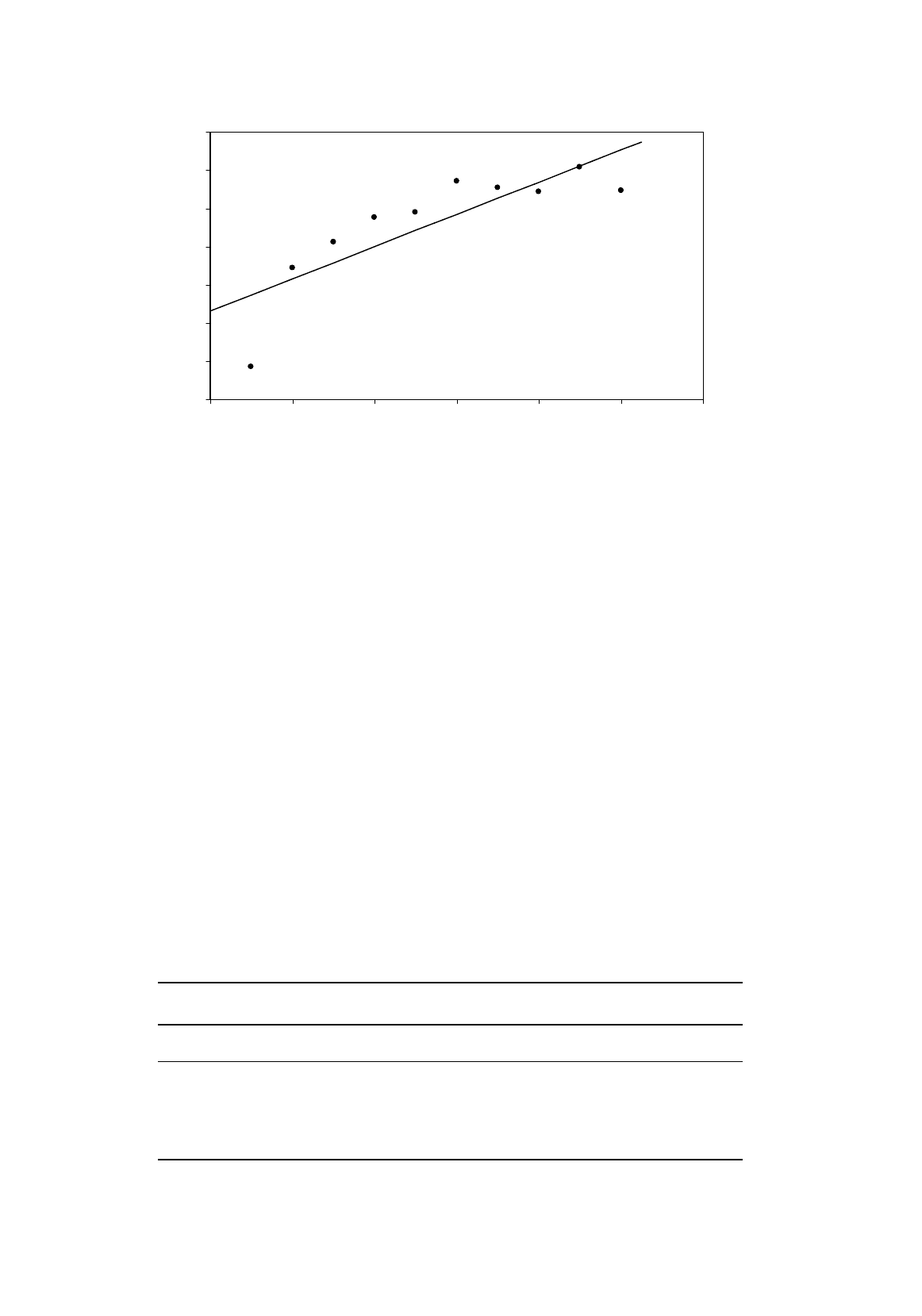
Figure 5.1.

Regression of expenditure on bananas on income

These observations are plotted in Figure 5.1, together with the line obtained by regressing Y on X

(standard errors in parentheses):

= 4.62 + 0.84XR

= 0.69 (5.7)

(1.26) (0.20)

Now, if you look at Figure 5.1, you will see that the regression line does not fit the observations

very well, despite the fact that the coefficient of income is significantly different from 0 at the 1

percent level. Quite obviously, the observations lie on a curve, while the regression equation is of

course a straight line. In this case, it is easy to see that the functional relationship between Y and X has

been misspecified. In the case of multiple regression analysis, nonlinearity might be detected using

the graphical technique described in Section 4.2. Alternatively, an examination of the residuals may

be sufficient to indicate that something is wrong. In this case the residuals are as shown in Table 5.2.

The residuals ought to be randomly positive or negative, large or small. Instead, they start out

being negative, cross to being positive, reach a maximum, fall again, and cross back to being negative:

very suspicious indeed.

ABLE

5.2

Household Y

e Household Y

1 1.71 5.46 –3.75 6 11.43 9.69 1.74

2 6.88 6.31 0.57 7 11.09 10.53 0.55

3 8.25 7.15 1.10 8 10.87 11.38 –0.51

4 9.52 8.00 1.52 9 12.15 12.22 –0.07

5 9.81 8.84 0.97 10 10.94 13.07 –2.13

024681012

Income ($ thousand)

Bananas (lbs)

TRANSFORMATIONS OF VARIABLES

The values of Y and X in this example were generated using the Monte Carlo technique, the true

relationship being

+−=

12 disturbance term, (5.8)

X taking the numbers from 1 to 10 and the values of the disturbance term being obtained using

normally distributed random numbers with 0 mean and standard deviation equal to 0.5.

If we realize this and define Z = 1/X, this equation becomes of the linear form (5.6). Z for each

household has already been calculated in Table 5.1. Regressing Y on Z, we obtain (standard errors in

parentheses):

= 12.48 – 10.99ZR

= 0.97 (5.9)

(0.26) (0.65)

Substituting Z = 1/X, this becomes

99.10

48.12

−=

(5.10)

In view of the excellent fit obtained with (5.9), it is not surprising that (5.10) is close to the true

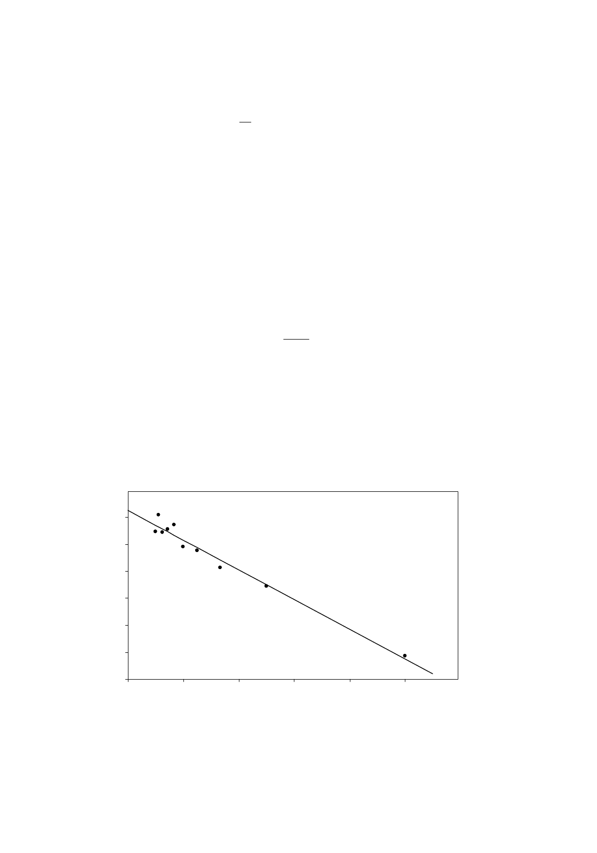
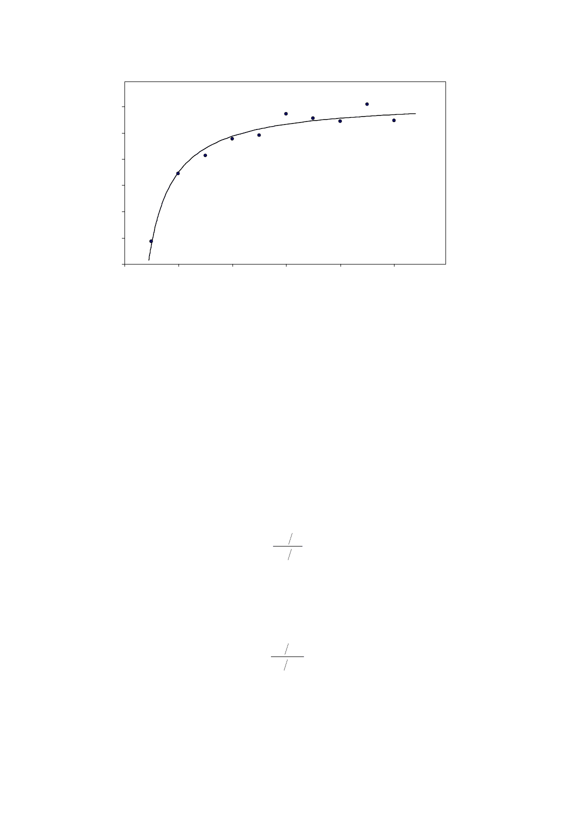
equation (5.8). The regression relationship, together with the observations on Y, X, and Z, is shown in

Figures 5.2 and 5.3. The improvement in the fit, as measured by R

, is clear from a comparison of

Figures 5.1 and 5.3.

Figure 5.2.

Regression of expenditure on bananas on the reciprocal of income

0 0.2 0.4 0.6 0.8 1

TRANSFORMATIONS OF VARIABLES

Figure 5.3.

Nonlinear regression of expenditure on bananas on income

5.2 Logarithmic Transformations

Next we will tackle functions such as (5.3), which are nonlinear in parameters as well as variables:

= (5.11)

When you see such a function, you can immediately say that the elasticity of Y with respect to X is

constant and equal to

. This is easily demonstrated. Regardless of the mathematical relationship

connecting Y and X, or the definitions of Y and X, the elasticity of Y with respect to X is defined to be

the proportional change in Y for a given proportional change in X:

elasticity

XdX

YdY

(5.12)

Thus, for example, if Y is demand and X is income, the above expression defines the income elasticity

of demand for the commodity in question.

The expression may be rewritten

elasticity

dXdY

(5.13)

In the case of the demand example, this may be interpreted as the marginal propensity to consume the

commodity divided by the average propensity to consume it.

0246810

TRANSFORMATIONS OF VARIABLES

If the relationship between Y and X takes the form (5.11),

−

. (5.14)

Hence

elasticity

===

dXdY

. (5.15)

Use of Logarithms

First, some basic rules:

1. If Y = XZ,log Y = log X + log Z

2. If Y = X/Z,log Y = log X – log Z

3. If Y = X

,log Y = n log X

These rules can be combined to transform more complicated expressions. For example,

take equation (5.11): if

log Y = log

+ log

X using Rule 1

= log

log X using Rule 3

Thus far we have not specified whether we are taking logarithms to base e or to base 10.

Throughout this text we shall be using e as the base, and so we shall be using what are

known as "natural" logarithms. This is standard in econometrics. Purists sometimes

write ln instead of log to emphasize that they are working with natural logarithms, but

this is now unnecessary. Nobody uses logarithms to base 10 anymore. They were

tabulated in the dreaded log tables that were universally employed for multiplying or

dividing large numbers until the early 1970s. When the pocket calculator was invented,

they became redundant. They are not missed.

With e as base, we can state another rule:

4. If Y = e

, log Y = X

, also sometimes written exp(X), is familiarly known as the antilog of X . One can say

that log e

is the log of the antilog of X, and since log and antilog cancel out, it is not

surprising that log e

turns out just to be X.

TRANSFORMATIONS OF VARIABLES

Thus, for example, if you see an Engel curve of the form

3.0

01.0

, (5.16)

this means that the income elasticity of demand is equal to 0.3. If you are trying to explain this to

someone who is not familiar with economic jargon, the easiest way to explain it is to say that a 1

percent change in

(income) will cause a 0.3 percent change in

(demand).

A function of this type can be converted into a linear equation by using logarithms. You will

certainly have encountered logarithms in a basic mathematics course. You probably thought that

when that course was finished, you could forget about them, writing them off as one of those academic

topics that never turn out to be of practical use. No such luck. In econometric work they are

indispensable, so if you are unsure about their use, you should review your notes from that basic math

course. The main properties of logarithms are given in a box.

In the box it is shown that (5.11) may be linearized as

log

= log

log

(5.17)

If we write

' = log

= log

, and

= log

, the equation may be rewritten

' =

(5.18)

The regression procedure is now as follows. First calculate

' and

for each observation, taking the

logarithms of the original data. Your regression application will almost certainly do this for you,

given the appropriate instructions. Second, regress

' on

. The coefficient of

will be a direct

estimate of

. The constant term will be an estimate of

, that is, of log

. To obtain an estimate

, you have to take the antilog, that is, calculate exp(

Example: Engel Curve

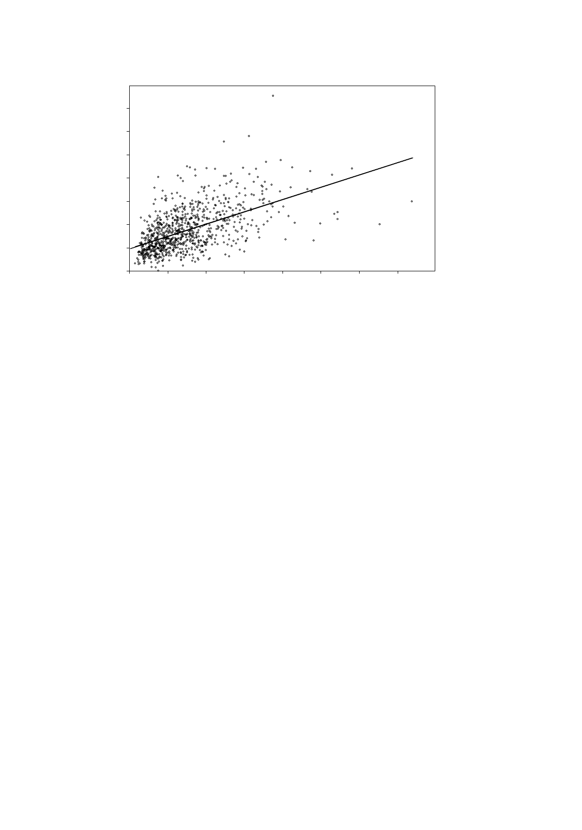
Figure 5.4 plots annual household expenditure on food eaten at home,

FDHO

, and total annual

household expenditure, both measured in dollars, for 869 representative households in the United

States in 1995, the data being taken from the Consumer Expenditure Survey.

When analyzing household expenditure data, it is usual to relate types of expenditure to total

household expenditure rather than income, the reason being that the relationship with expenditure

tends to be more stable than that with income. The outputs from linear and logarithmic regressions are

shown.

The linear regression indicates that 5.3 cents out of the marginal dollar are spent on food eaten at

home. Interpretation of the intercept is problematic because literally it implies that $1,916 would be

spent on food eaten at home even if total expenditure were 0.

TRANSFORMATIONS OF VARIABLES

Figure 5.4.

Regression of expenditure on food eaten

at home on total household expenditure

. reg FDHO EXP

Source | SS df MS Number of obs = 869

---------+------------------------------ F( 1, 867) = 381.47

Model | 915843574 1 915843574 Prob > F = 0.0000

Residual | 2.0815e+09 867 2400831.16 R-squared = 0.3055

---------+------------------------------ Adj R-squared = 0.3047

Total | 2.9974e+09 868 3453184.55 Root MSE = 1549.5

------------------------------------------------------------------------------

FDHO | Coef. Std. Err. t P>|t| [95% Conf. Interval]

---------+--------------------------------------------------------------------

EXP | .0528427 .0027055 19.531 0.000 .0475325 .0581529

_cons | 1916.143 96.54591 19.847 0.000 1726.652 2105.634

------------------------------------------------------------------------------

. g LGFDHO = ln(FDHO)

. g LGEXP = ln(EXP)

. reg LGFDHO LGEXP

Source | SS df MS Number of obs = 868

---------+------------------------------ F( 1, 866) = 396.06

Model | 84.4161692 1 84.4161692 Prob > F = 0.0000

Residual | 184.579612 866 .213140429 R-squared = 0.3138

---------+------------------------------ Adj R-squared = 0.3130

Total | 268.995781 867 .310260416 Root MSE = .46167

------------------------------------------------------------------------------

LGFDHO | Coef. Std. Err. t P>|t| [95% Conf. Interval]

---------+--------------------------------------------------------------------

LGEXP | .4800417 .0241212 19.901 0.000 .4326988 .5273846

_cons | 3.166271 .244297 12.961 0.000 2.686787 3.645754

------------------------------------------------------------------------------

2000

4000

6000

8000

10000

12000

14000

0 20000 40000 60000 80000 100000 120000 140000

FDHO

EXP

TRANSFORMATIONS OF VARIABLES

Figure 5.5.

Logarithmic regression of expenditure on food eaten

at home on total household expenditure

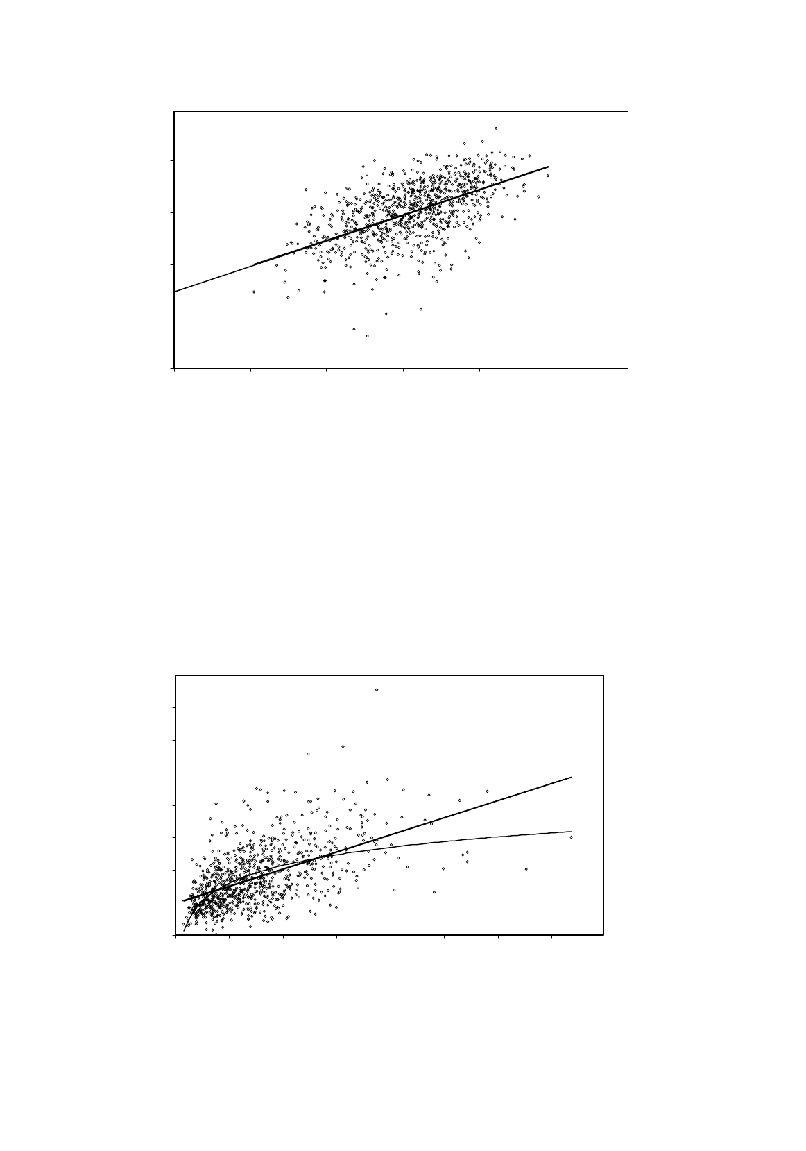
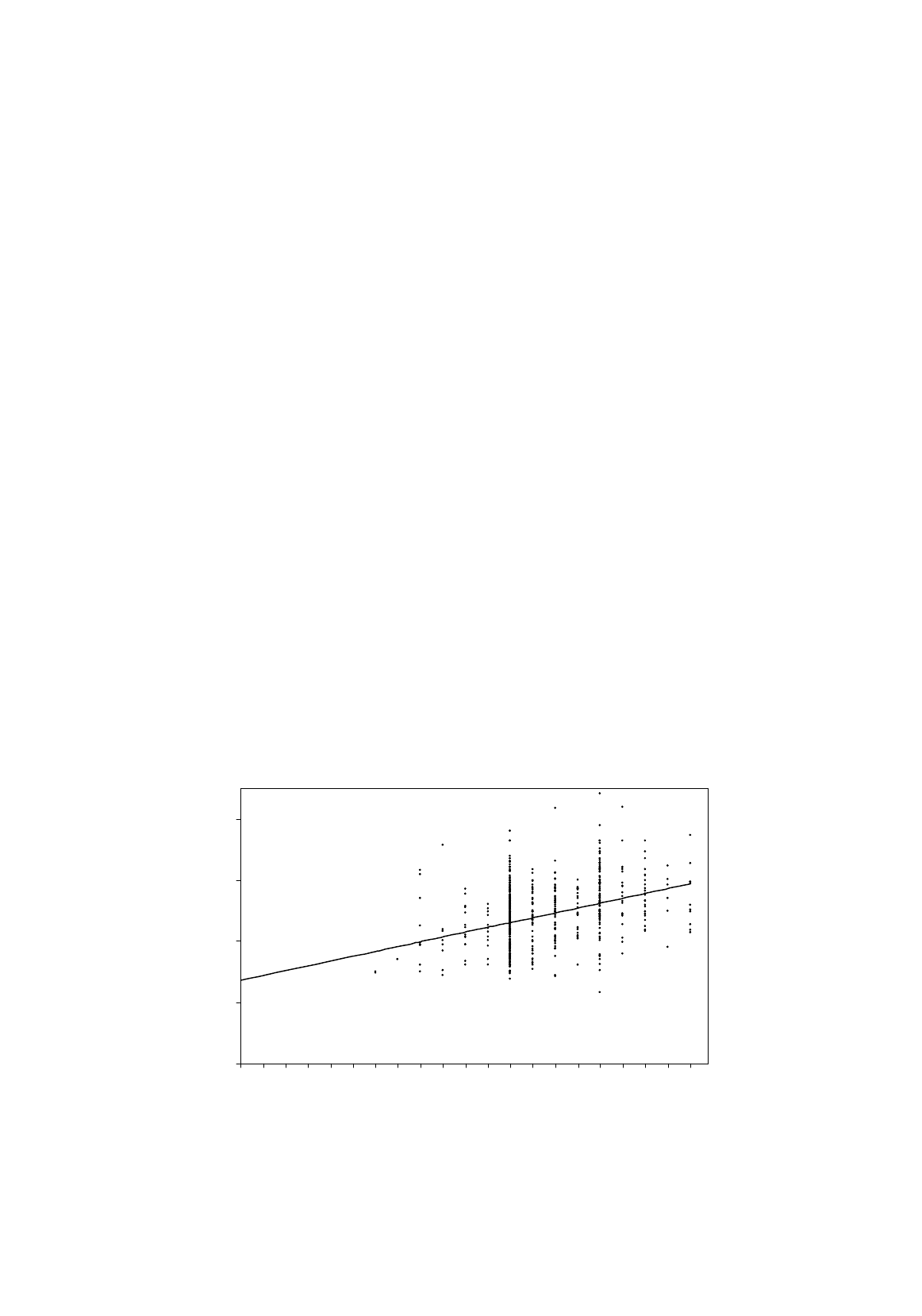
The logarithmic regression, shown in Figure 5.5, indicates that the elasticity of expenditure on

food eaten at home with respect to total household expenditure is 0.48. Is this figure plausible? Yes,

because food eaten at home is a necessity rather than a luxury, so one would expect the elasticity to be

less than 1. The intercept has no economic meaning. Figure 5.6 plots the logarithmic regression line

in the original diagram. While there is not much difference between the regression lines over the

middle part of the range of observations, it is clear that the logarithmic regression gives a better fit for

very low and very high levels of household expenditure.

Figure 5.6.

Linear and logarithmic regressions of expenditure on food

eaten at home on total household expenditure

2000

4000

6000

8000

10000

12000

14000

0 20000 40000 60000 80000 100000 120000 140000

FDHO

EXP

789101112

LGFDHO

LGEXP

TRANSFORMATIONS OF VARIABLES

Semi-Logarithmic Models

Another common functional form is given by equation (5.18):

, (5.19)

Here

should be interpreted as the proportional change in

per

unit

change in

. Again, this is

easily demonstrated. Differentiating,

221

, (5.20)

Hence

dXdY

. (5.21)

In practice it is often more natural to speak of the percentage change in

, rather than the proportional

change, per unit change in

, in which case one multiplies the estimate of

by 100.

The function can be converted into a model that is linear in parameters by taking the logarithms

of both sides:

eeY

log

loglog

loglogloglog

ββ

+==

(5.22)

Note that only the left side is logarithmic in variables, and for this reason the model is described as

semi-logarithmic.

The interpretation of

as the proportional change in

per

unit

change in

is valid only when

is small. When

is large, the interpretation may be a little more complex. Suppose that

is related

by (5.18) and that

increases by one unit to

'. Then

', the new value of

is given by

...)

)1(

222

+++=

βββ

ββ

Yeee

eeY

(5.23)

Thus the proportional change per unit change in

is actually greater than

. However, if

is small

(say, less than 0.1),

and further terms will be very small and can be neglected. In that case, the

right side of the equation simplifies to

(1 +

) and the original marginal interpretation of

still

applies.

TRANSFORMATIONS OF VARIABLES

Example: Semi-Logarithmic Earnings Function

For fitting earnings functions, the semi-logarithmic model is generally considered to be superior to the

linear model. We will start with the simplest possible version:

eEARNINGS

, (5.24)

where

EARNINGS

is hourly earnings, measured in dollars, and

is years of schooling. After taking

logarithms, the model becomes

. reg LGEARN S

Source | SS df MS Number of obs = 570

---------+------------------------------ F( 1, 568) = 93.21

Model | 21.681253 1 21.681253 Prob > F = 0.0000

Residual | 132.12064 568 .23260676 R-squared = 0.1410

---------+------------------------------ Adj R-squared = 0.1395

Total | 153.801893 569 .270302096 Root MSE = .48229

------------------------------------------------------------------------------

LGEARN | Coef. Std. Err. t P>|t| [95% Conf. Interval]

---------+--------------------------------------------------------------------

S | .0792256 .0082061 9.655 0.000 .0631077 .0953435

_cons | 1.358919 .1127785 12.049 0.000 1.137406 1.580433

------------------------------------------------------------------------------

LGEARN

(5.25)

where

LGEARN

is the natural logarithm of

EARNINGS

and

is the logarithm of

Figure 5.7.

Semi-logarithmic regression of earnings on schooling

0 1 2 3 4 5 6 7 8 9 10 11 12 13 14 15 16 17 18 19 20

Years of schooling (highest grade completed)

Logarithm of hourly earnings

TRANSFORMATIONS OF VARIABLES

Figure 5.8.

Linear and semi-logarithmic regressions of earnings on schooling

The regression output, which uses EAEF Data Set 21, indicates that every extra year of schooling

increases earnings by a proportion 0.079, that is, 7.9 percent, as a first approximation. Strictly

speaking, a whole extra year of schooling is not marginal, so it would be more accurate to calculate

0.079

, which is 1.082. Thus a more accurate interpretation is that an extra year of schooling raises

earnings by 8.2 percent.

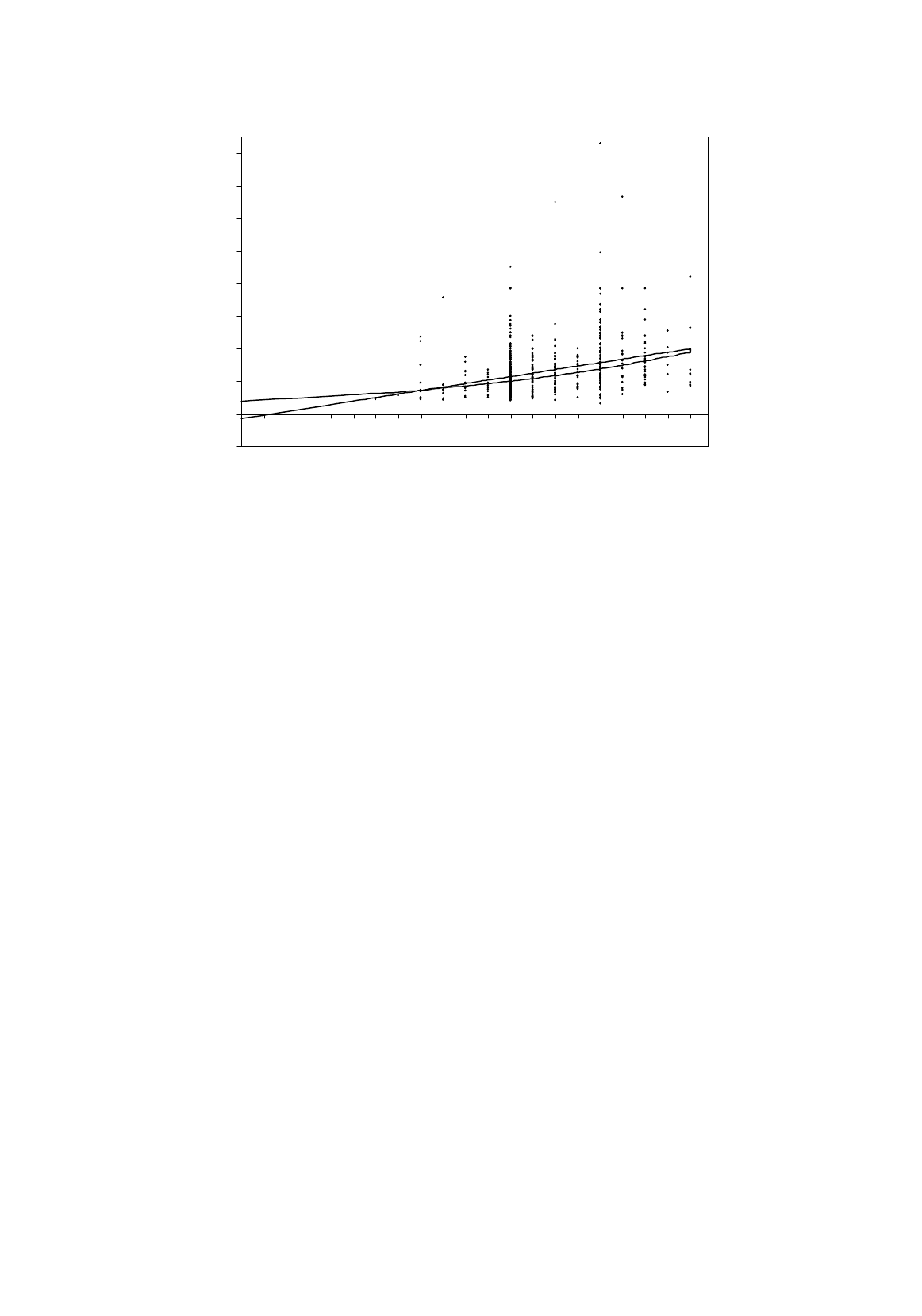
The scatter diagram for the semi-logarithmic regression is shown in Figure 5.7. For the purpose

of comparison, it is plotted together with the linear regression in a plot with the untransformed

variables in Figure 5.8. The two regression lines do not differ greatly in their overall fit, but the semi-

logarithmic specification has the advantages of not predicting negative earnings for individuals with

low levels of schooling and of allowing the increase in earnings per year of schooling to increase with

schooling.

Exercises

Note: For all of these exercises, you should discuss the plausibility of the estimated coefficients.

5.1

Download the CES data set from the website and fit linear and (double) logarithmic regressions

for your commodity, excluding observations with 0 expenditure on your commodity. Interpret

the regressions and perform appropriate tests.

5.2

Repeat the logarithmic regression in Exercise 5.1, adding the logarithm of the size of the

household as an additional explanatory variable. Interpret the results and perform appropriate

tests.

5.3

Using your EAEF data set, regress the (natural) logarithm of WEIGHT85 on the logarithm of

HEIGHT. Interpret the regression results and perform appropriate tests.

5.4

Using your EAEF data set, regress the logarithm of earnings on S and ASVABC. Interpret the

-10

0 1 2 3 4 5 6 7 8 9 1011121314151617181920

Years of schooling (hghest grade completed)

Hourly earnings ($)