Dougherty С. Introduction to Econometrics, 3Ed

Подождите немного. Документ загружается.

DUMMY VARIABLES

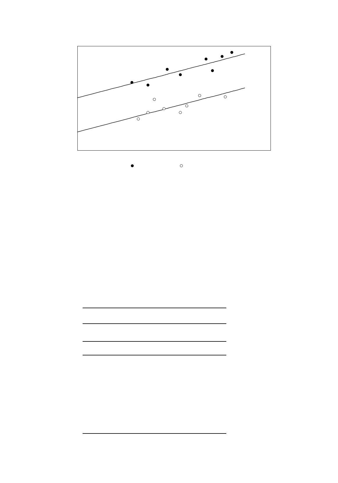
Figure 6.1.

Cost functions for regular and occupational schools

The object of the present exercise is to estimate this unknown shift factor, and we shall do this by

introducing what is known as a dummy variable. We shall rewrite the model

COST =

OCC +

N + u (6.6)

where OCC is a dummy variable, an artificial variable with two possible values, 0 and 1. If OCC is

equal to 0, the cost function becomes (6.3), that for regular schools. If OCC is equal to 1, the cost

function becomes (6.5), that for occupational schools. Hence, instead of two separate regressions for

the different types of school, we can run just one regression using the whole sample. Using the whole

ABLE

6.1

Recurrent Expenditure, Number

of Students, and Type of School

School Type COST N OCC

1 Occupational 345,000 623 1

2 Occupational 537,000 653 1

3 Regular 170,000 400 0

4 Occupational 526,000 663 1

5 Regular 100,000 563 0

6 Regular 28,000 236 0

7 Regular 160,000 307 0

8 Occupational 45,000 173 1

9 Occupational 120,000 146 1

10 Occupational 61,000 99 1

COST

Occupational schools Re

ular schools

DUMMY VARIABLES

sample in a single regression will reduce the population variances of the coefficients, and this should

be reflected by smaller standard errors. We will also obtain a single estimate of

, instead of two

separate ones that are likely to conflict. The price we have to pay is that we have to assume that

the same for both subsamples. We will relax this assumption in due course.

Data for the first 10 schools in the sample are shown in Table 6.1. Note how OCC varies with the

type of school.

. reg COST N OCC

Source | SS df MS Number of obs = 74

---------+------------------------------ F( 2, 71) = 56.86

Model | 9.0582e+11 2 4.5291e+11 Prob > F = 0.0000

Residual | 5.6553e+11 71 7.9652e+09 R-squared = 0.6156

---------+------------------------------ Adj R-squared = 0.6048

Total | 1.4713e+12 73 2.0155e+10 Root MSE = 89248

------------------------------------------------------------------------------

COST | Coef. Std. Err. t P>|t| [95% Conf. Interval]

---------+--------------------------------------------------------------------

N | 331.4493 39.75844 8.337 0.000 252.1732 410.7254

OCC | 133259.1 20827.59 6.398 0.000 91730.06 174788.1

_cons | -33612.55 23573.47 -1.426 0.158 -80616.71 13391.61

------------------------------------------------------------------------------

The data are fed into the computer regression program and multiple regression is used to regress

COST on N and OCC. OCC is treated exactly like an ordinary variable, even though it consists only

of 0s and 1s.

The Stata output gives the results of the regression, using the full sample of 74 schools. In

equation form, we have (standard errors in parentheses):

STOC

= –34,000 + 133,000OCC + 331N. R

= 0.62 (6.7)

(24,000) (21,000) (40)

Putting OCC equal to 0 and 1, respectively, we can obtain the implicit cost functions for the two

types of school.

Regular schools:

STOC

= –34,000 + 331N (6.8)

Occupational schools:

STOC

= –34,000 + 133,000 + 331N = 99,000 + 331N (6.9)

The regression implies that the marginal cost per student per year is 331 yuan and that the annual

overhead cost of a regular school is –34,000 yuan. Obviously having a negative intercept does not

make any sense at all and it suggests that the model is misspecified in some way. We will come back

to this later. The coefficient of the dummy variable, 133,000, is an estimate of the extra annual

overhead cost of an occupational school. The marginal cost of an occupational school is the same as

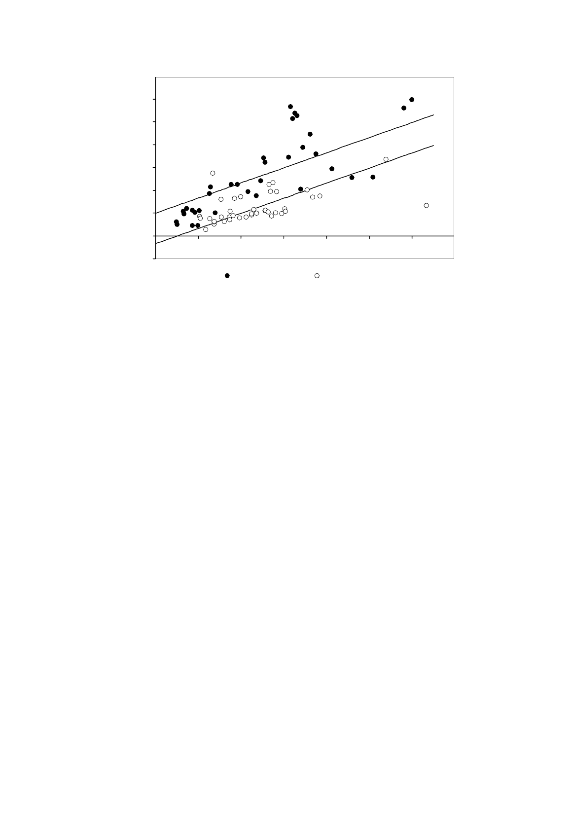
that for a regular school – it must be, given the model specification. Figure 6.2 shows the data and the

cost functions derived from the regression results.

DUMMY VARIABLES

Figure 6.2.

Cost functions for regular and occupational schools in Shanghai

Standard Errors and Hypothesis Testing

In addition to the estimates of the coefficients, the regression results include standard errors and the

usual diagnostic statistics. We will perform a t test on the coefficient of the dummy variable. Our null

hypothesis is H

= 0 and our alternative hypothesis is H

≠

0. In words, our null hypothesis is

that there is no difference in the overhead costs of the two types of school. The t statistic is 6.40, so it

is rejected at the 0.1 percent significance level. We can perform t tests on the other coefficients in the

usual way. The t statistic for the coefficient of N is 8.34, so we conclude that the marginal cost is

(very) significantly different from 0. In the case of the intercept, the t statistic is –1.43, so we do not

reject the null hypothesis H

= 0. Thus one explanation of the nonsensical negative overhead cost

of regular schools might be that they do not actually have any overheads and our estimate is a random

number. A more realistic version of this hypothesis is that

is positive but small (as you can see, the

95 percent confidence interval includes positive values) and the disturbance term is responsible for the

negative estimate. As already noted, a further possibility is that the model is misspecified in some

way.

Exercises

6.1

Using your EAEF data set, regress S on ASVABC, SM, SF and MALE, a dummy variable that is

1 for male respondents and 0 for female ones. Interpret the coefficients and perform t tests. Is

there any evidence that the educational attainment of males is different from that of females?

6.2*

The Stata output shows the result of regressing weight on height, first with a linear

specification, then with a double-logarithmic one, including a dummy variable MALE, defined

as in Exercise 6.1, in both cases. Give an interpretation of the equations and perform

appropriate statistical tests.

COST

-100000

100000

200000

300000

400000

500000

600000

0 200 400 600 800 1000 1200

Occupational schools Regular schools

DUMMY VARIABLES

. g LGWEIGHT=ln(WEIGHT85)

(20 missing values generated)

. g LGHEIGHT=ln(HEIGHT)

(19 missing values generated)

. reg WEIGHT85 HEIGHT MALE

Source | SS df MS Number of obs = 550

---------+------------------------------ F( 2, 547) = 179.27

Model | 252465.351 2 126232.675 Prob > F = 0.0000

Residual | 385164.642 547 704.140113 R-squared = 0.3959

---------+------------------------------ Adj R-squared = 0.3937

Total | 637629.993 549 1161.43897 Root MSE = 26.536

------------------------------------------------------------------------------

WEIGHT85 | Coef. Std. Err. t P>|t| [95% Conf. Interval]

---------+--------------------------------------------------------------------

HEIGHT | 4.389971 .4313611 10.177 0.000 3.542644 5.237298

MALE | 10.74783 3.408249 3.153 0.002 4.05297 17.44269

_cons | -147.6628 27.9497 -5.283 0.000 -202.5647 -92.76089

------------------------------------------------------------------------------

. reg LGWEIGHT LGHEIGHT MALE

Source | SS df MS Number of obs = 550

---------+------------------------------ F( 2, 547) = 216.63

Model | 10.9693142 2 5.48465712 Prob > F = 0.0000

Residual | 13.8491387 547 .025318352 R-squared = 0.4420

---------+------------------------------ Adj R-squared = 0.4399

Total | 24.8184529 549 .045206654 Root MSE = .15912

------------------------------------------------------------------------------

LGWEIGHT | Coef. Std. Err. t P>|t| [95% Conf. Interval]

---------+--------------------------------------------------------------------

LGHEIGHT | 1.901986 .1747121 10.886 0.000 1.558797 2.245174

MALE | .077839 .020447 3.807 0.000 .0376748 .1180032

_cons | -3.033228 .7283617 -4.164 0.000 -4.463957 -1.6025

------------------------------------------------------------------------------

6.3

Using your EAEF data set, regress LGEARN on S, ASVABC and MALE. Interpret the

coefficients and perform t tests. (See Section 3 of the EAEF manual for help with the

interpretation of the coefficient of a dummy variable in a semi-logarithmic regression.)

6.2 Extension to More than Two Categories and to Multiple Sets of Dummy Variables

In the previous section we used a dummy variable to differentiate between regular and occupational

schools when fitting a cost function. In actual fact there are two types of regular secondary school in

Shanghai. There are general schools, which provide the usual academic education, and vocational

schools. As their name implies, the vocational schools are meant to impart occupational skills as well

as give an academic education. However the vocational component of the curriculum is typically

quite small and the schools are similar to the general schools. Often they are just general schools with

a couple of workshops added. Likewise there are two types of occupational school. There are

technical schools training technicians and skilled workers’ schools training craftsmen.

Thus now the qualitative variable has four categories and we need to develop a more elaborate set

of dummy variables. The standard procedure is to choose one category as the reference category to

DUMMY VARIABLES

ABLE

6.2

Recurrent Expenditure, Number of Students, and Type of School

School Type COST N TECH WORKER VOC

1 Technical 345,000 623 1 0 0

2 Technical 537,000 653 1 0 0

3 General 170,000 400 0 0 0

4 Skilled workers' 526,000 663 0 1 0

5 General 100,000 563 0 0 0

6 Vocational 28,000 236 0 0 1

7 Vocational 160,000 307 0 0 1

8 Technical 45,000 173 1 0 0

9 Technical 120,000 146 1 0 0

10 Skilled workers' 61,000 99 0 1 0

which the basic equation applies, and then to define dummy variables for each of the other categories.

In general it is good practice to select the dominant or most normal category, if there is one, as the

reference category. In the Shanghai sample it is sensible to choose the general schools. They are the

most numerous and the other schools are variations of them.

Accordingly we will define dummy variables for the other three types. TECH will be the dummy

variable for the technical schools: TECH is equal to 1 if the observation relates to a technical school, 0

otherwise. Similarly we will define dummy variables WORKER and VOC for the skilled workers’

schools and the vocational schools. The regression model is now

COST =

TECH +

WORKER +

VOC +

N + u (6.10)

where

, and

are coefficients that represent the extra overhead costs of the technical, skilled

workers’, and vocational schools, relative to the cost of a general school. Note that you do not include

a dummy variable for the reference category, and that is the reason that the reference category is

usually described as the omitted category. Note that we do not make any prior assumption about the

size, or even the sign, of the

coefficients. They will be estimated from the sample data.

Table 6.2 gives the data for the first 10 of the 74 schools. Note how the values of the dummy

variables TECH, WORKER, and VOC are determined by the type of school in each observation.

. reg COST N TECH WORKER VOC

Source | SS df MS Number of obs = 74

---------+------------------------------ F( 4, 69) = 29.63

Model | 9.2996e+11 4 2.3249e+11 Prob > F = 0.0000

Residual | 5.4138e+11 69 7.8461e+09 R-squared = 0.6320

---------+------------------------------ Adj R-squared = 0.6107

Total | 1.4713e+12 73 2.0155e+10 Root MSE = 88578

------------------------------------------------------------------------------

COST | Coef. Std. Err. t P>|t| [95% Conf. Interval]

---------+--------------------------------------------------------------------

N | 342.6335 40.2195 8.519 0.000 262.3978 422.8692

TECH | 154110.9 26760.41 5.759 0.000 100725.3 207496.4

WORKER | 143362.4 27852.8 5.147 0.000 87797.57 198927.2

VOC | 53228.64 31061.65 1.714 0.091 -8737.646 115194.9

_cons | -54893.09 26673.08 -2.058 0.043 -108104.4 -1681.748

------------------------------------------------------------------------------

DUMMY VARIABLES

The Stata output gives the regression results for this model. In equation form, we have (standard

errors in parentheses):

STOC

= –55,000 + 154,000

TECH

+ 143,000

WORKER

+53,000

VOC

+ 343

=0.63 (6.11)

(27,000) (27,000) (28,000) (31,000) (40)

The coefficient of

indicates that the marginal cost per student per year is 343 yuan. The

constant indicates that the annual overhead cost of a general academic school is –55,000 yuan per

year. Obviously this is nonsense and indicates that something is wrong with the model. The

coefficients of

TECH

WORKER

, and

VOC

indicate that the overhead costs of technical, skilled

workers’, and vocational schools are 154,000 yuan, 143,000 yuan, and 53,000 yuan greater than the

cost of a general school.

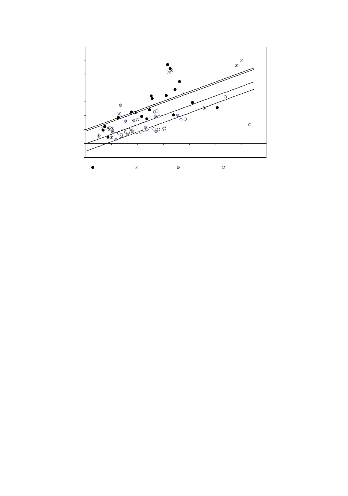
From this equation we can obtain the implicit cost functions shown in the following diagram for

the four types of school. First, putting the three dummy variables equal to 0, we obtain the cost

function for general schools:

General schools

STOC

= –55,000 + 343

(6.12)

Next, putting

TECH

equal to 1 and

WORKER

and

VOC

to 0, we obtain the cost function for technical

schools:

Technical schools

STOC

= –55,000 + 154,000 + 343

= 99,000 + 343

(6.13)

And similarly we obtain the cost functions for skilled workers’ and vocational schools:

Skilled workers’ schools

STOC

= –55,000 + 143,000 + 343

= 88,000 + 343

(6.14)

Vocational schools

STOC

= –55,000 + 53,000 + 343

= –2,000 + 343

(6.15)

Note that in each case the annual marginal cost per student is estimated at 343 yuan. The model

specification assumes that this figure does not differ according to type of school. The four cost

functions are illustrated in Figure 6.3.

DUMMY VARIABLES

Figure 6.3.

We can perform t tests on the coefficients in the usual way. The t statistic for N is 8.52, so the

marginal cost is (very) significantly different from 0, as we would expect. The t statistic for the

technical school dummy is 5.76, indicating that the annual overhead cost of a technical school is (very)

significantly greater than that of a general school, again as expected. Similarly for skilled workers’

schools, the t statistic being 5.15. In the case of vocational schools, however, the t statistic is only

1.71, indicating that the overhead cost of such a school is not significantly greater than that of a

general school. This is not surprising, given that the vocational schools are not much different from

the general schools. Note that the null hypotheses for the tests on the coefficients of the dummy

variables are that the overhead costs of the other schools are not different from the overhead cost of a

general school.

Joint Explanatory Power of a Group of Dummy Variables

Finally we will perform an F test of the joint explanatory power of the dummy variables as a

group. The null hypothesis is H

= 0. The alternative hypothesis H

is that at least one

is different from 0. The residual sum of squares in the specification including the dummy variables is

5.41×10

. (In the Stata output, it appears as 5.4138e+11. The e+11 means that the coefficient should

be multiplied by 10

.) The residual sum of squares in the original specification excluding the dummy

variables was 8.92×10

(see Section 6.1). The reduction in RSS when we include the dummies is

therefore (8.92 - 5.41)×10

. We will check whether this reduction is significant with the usual F test.

The numerator in the F ratio is the reduction in RSS divided by the cost, which is the 3 degrees of

freedom given up when we estimate three additional coefficients (the coefficients of the dummies).

The denominator is RSS for the specification including the dummy variables, divided by the number of

degrees of freedom remaining after they have been added. The F ratio is therefore given by

COST

-100000

100000

200000

300000

400000

500000

600000

0 200 400 600 800 1000 1200

Technical schools Workers' schools Vocational schools General schools

DUMMY VARIABLES

9.14

07846.0

1674.1

69104138.5

3)104138.5109160.8(

)69,3(

1111

×−×

(6.16)

Note that the ratios were calculated to four significant figures. This will ensure that the F statistic will

be correct to three significant figures. The critical value of F(3,69) will be a little below 6.17, the

critical value for F(3,60) at the 0.1 percent significance level, so we can reject H

at this level. This is

only to be expected because t tests showed that

and

were both significantly different from 0, and

it is rare (but not impossible) for the F test not to reject H

when one or more coefficients is

significant.

The Dummy Variable Trap

What would happen if you included a dummy variable for the reference category? There would be

two consequences. First, were it possible to compute regression coefficients, you would not be able to

give them an interpretation. The coefficient b

is a basic estimate of the intercept, and the coefficients

of the dummies are the estimates of the increase in the intercept from this basic level, but now there is

no definition of what is basic, so the interpretation collapses. The other consequence is that the

numerical procedure for calculating the regression coefficients will break down and the computer will

simply send you an error message (or possibly, in sophisticated applications, drop one of the dummies

for you). Suppose that there are m dummy categories and you define dummy variables D

, ..., D

Then, in observation i,

∑

= 1 because one of the dummy variables will be equal to 1 and all the

others will be equal to 0. But the intercept

is really the product of the parameter

and a special

variable whose value is 1 in all observations (see the box in Section 4.2). Hence, for all observations,

the sum of the dummy variables is equal to this special variable, and one has an exact linear

relationship among the variables in the regression model. As a consequence the model is subject to a

special case of exact multicollinearity, making it impossible to compute regression coefficients..

Change of Reference Category

The skilled workers' schools are considerably less academic than the others, even the technical

schools. Suppose that we wish to investigate whether their costs are significantly different from the

others. The easiest way to do this is to make them the omitted category (reference category). Then

the coefficients of the dummy variables become estimates of the differences between the overhead

costs of the other types of school and those of the skilled workers' schools. Since skilled workers'

schools are now the reference category, we need a dummy variable, which will be called GEN, for the

general academic schools. The model becomes

COST =

TECH +

VOC +

GEN +

N + u (6.17)

where

, and

are the extra costs of technical, vocational, and general schools relative to skilled

workers’ schools. The data table for the first 10 schools is now as shown in Table 6.3. The Stata

output is shown.

DUMMY VARIABLES

ABLE

6.3

Recurrent Expenditure, Enrolments and Type of School

School Type COST N TECH GEN VOC

1 Technical 345,000 623 1 0 0

2 Technical 537,000 653 1 0 0

3 General 170,000 400 0 1 0

4 Skilled workers' 526,000 663 0 0 0

5 General 100,000 563 0 1 0

6 Vocational 28,000 236 0 0 1

7 Vocational 160,000 307 0 0 1

8 Technical 45,000 173 1 0 0

9 Technical 120,000 146 1 0 0

10 Skilled workers' 61,000 99 0 0 0

. reg COST N TECH VOC GEN

Source | SS df MS Number of obs = 74

---------+------------------------------ F( 4, 69) = 29.63

Model | 9.2996e+11 4 2.3249e+11 Prob > F = 0.0000

Residual | 5.4138e+11 69 7.8461e+09 R-squared = 0.6320

---------+------------------------------ Adj R-squared = 0.6107

Total | 1.4713e+12 73 2.0155e+10 Root MSE = 88578

------------------------------------------------------------------------------

COST | Coef. Std. Err. t P>|t| [95% Conf. Interval]

---------+--------------------------------------------------------------------

N | 342.6335 40.2195 8.519 0.000 262.3978 422.8692

TECH | 10748.51 30524.87 0.352 0.726 -50146.93 71643.95

VOC | -90133.74 33984.22 -2.652 0.010 -157930.4 -22337.07

GEN | -143362.4 27852.8 -5.147 0.000 -198927.2 -87797.57

_cons | 88469.29 28849.56 3.067 0.003 30916.01 146022.6

------------------------------------------------------------------------------

The regression equation is therefore (standard errors in parentheses):

STOC

= 88,000 + 11,000TECH – 143,000GEN – 90,000VOC + 343NR

=0.63 (6.18)

(29,000) (30,000) (28,000) (34,000) (40)

From this equation we can again obtain the implicit cost functions shown in the following diagram for

the four types of school. Putting all the dummy variables equal to 0, we obtain the cost function for

skilled workers’ schools:

Skilled workers’ schools:

STOC

= 88,000 + 343N (6.19)

Then, putting TECH, WORKER, and GEN equal to 1 and the other two to 0, we derive the cost

functions for the other types of school:

Technical schools:

STOC

= 88,000 + 11,000 + 343N = 99,000 + 343N (6.20)

Vocational schools:

STOC

= 88,000 – 90,000 + 343N = –2,000 + 343N (6.21)

DUMMY VARIABLES

General schools:

STOC

= 88,000 – 143,000 + 343N = –55,000 + 343N (6.22)

Note that these equations are identical to those obtained when general schools were the reference

category. The choice of omitted category does not affect the substance of the regression results. The

only components that change are the standard errors and the interpretation of the t tests. R

, the

coefficients of the other variables, the t statistics for the other variables, and the F statistic for the

equation as a whole do not alter. And of course the diagram representing the four cost functions is the

same as before.

Multiple Sets of Dummy Variables

It may happen that you wish to include more than one set of dummy variables in your regression

equation. This is especially common when working with cross-section data, when you may have

gathered data on a number of qualitative as well as quantitative characteristics. There is no problem in

extending the use of dummy variables in this way, provided that the framework is defined clearly.

We will illustrate the procedure using the school cost data. Many of the occupational schools and

some of the regular schools are residential. We will investigate the extra cost of running a residential

school, controlling for number of students and type of school. To do this, we introduce a dummy

variable, RES, which is equal to 1 for residential schools and 0 for the others. For the sake of

simplicity we will revert to the occupational/regular classification of school type. The model now

becomes

COST =

OCC +

RES +

N + u (6.23)

where

is the extra cost of a residential school. The reference category now has two dimensions, one

for each qualitative characteristic. In this case it is a nonresidential (RES = 0), regular (OCC = 0)

school. Table 6.4 presents the data for the first 10 schools in the sample. The second, fourth and

seventh are residential schools and so RES is set equal to 1, while for the others it is 0.

ABLE

6.4

Recurrent Expenditure, Number of Students,

School Type and Whether Residential

School Type COST N OCC RES

1 Occupational, nonresidential 345,000 623 1 0

2 Occupational, residential 537,000 653 1 1

3 Regular, nonresidential 170,000 400 0 0

4 Occupational, residential 526,000 663 1 1

5 Regular, nonresidential 100,000 563 0 0

6 Regular, nonresidential 28,000 236 0 0

7 Regular, residential 160,000 307 0 1

8 Occupational, nonresidential 45,000 173 1 0

9 Occupational, nonresidential 120,000 146 1 0

10 Occupational, nonresidential 61,000 99 1 0