Deza M.M., Laurent M. Geometry of Cuts and Metrics

52

Chapter

4.

The

Cut

Cone

and

iI-Metrics

which

can

be easily

brought

in

the

form (4.5.1).

Thus,

we find

an

instance

of

the

max-cut

problem.

As

the

interaction

Jij

decreases

rapidly

as

the

distance

Tij

increases,

it

is

common

to

set

Jij

:=

0

if

the

atoms

are far

apart.

Moreover,

there

are two

ways

of

generating

the

interactions

Jij

that

have

been

intensively

studied:

the

Gaussian

model

where

the

Jij's

are chosen from a

Gaussian

distribution,

and

the

±J-model

where interactions take only two values

±J

(according

to

some

distribution).

One

also assumes

that

the

atoms

are regularly

located

on

a

2-

or

3-dimensional

grid;

then

interactions between

atoms

are

nonzero only along

the

edges

of

the

grid.

In

this

model,

the

problem

of

determining

ground

states

of

the

spin

glass

system

is

formulated

as a

max-cut

problem

on

a

graph

which is a

2-dimensional or 3-dimensional

grid

plus

a universal

node

(corresponding

to

the

exterior

magnetic

field)

joined

to

all nodes

in

the

grid.

This

instance

of

the

max-cut

problem

is

NP-hard,

as

mentioned

earlier in

Section

4.4.

In

fact,

if

one neglects

the

exterior magnetic field,

the

problem

remains

NP-hard

in

the

3-dimensional case

(Barahona

[1982]),

but

it

becomes

polynomial

in

the

2-dimensional case (since a 2-dimensional

grid

is a

planar

graph).

Interestingly,

the

classical technique used for solving

max-cut

on

a

planar

graph

(reduction

to

a Chinese

postman

problem

in

the

dual

graph)

by Orlova

and

Dorfman

[1972]

and

Hadlock [1975]) was

independently

discovered

in

the

field

of

physics by Toulouse [1977].

Toulouse's

paper

together

with

the

papers

by Bieche,

Maynard,

Rammal

and

Uhry

[1980]

and

by

Barahona,

Maynard,

Rammal

and

Uhry

[1982]

have

pioneered

the

study

of

spin

glasses from

an

optimization

point

of

view. Since

then,

lots

of

efforts have

been

made

for designing algorithms

permitting

to

com-

pute

exact

ground

states

of

spin

glass systems, in

the

various cases

mentioned

above.

These

algorithms

are essentially

of

the

type

'branch-and-cut'

and

use

knowledge

of

the

cut

polytope

(in

particular,

the

cycle inequalities

presented

in Section 27.3.1).

Computational

results

can

be

found in Grotschel,

Junger

and

Reinelt [1987],

Barahona,

Grotschel,

Junger

and

Reinelt [1988],

Barahona,

Junger

and

Reinelt [1989],

Barahona

[1994]'

De

Simone, Diehl,

Junger,

Mutzel,

Reinelt

and

Rinaldi

[1995, 1996]

and

in references therein.

M.M. Deza, M. Laurent, Geometry of Cuts and Metrics, Algorithms and Combinatorics 15,

DOI 10.1007/978-3-642-04295-9_5, © Springer-Verlag Berlin Heidelberg 2010

Chapter

5.

The

Correlation

Cone

and

{O,l}-Covariances

We

introduce

here

another

set of polyhedra:

the

correlation cone

and

the

corre-

lation

polytope,

that

have

been

considered in

the

literature

in connection

with

several different

problems

(relevant,

among

others,

to

probability

theory,

quan-

tum

logic, or

optimization).

The

correlation

polyhedra

turn

out

to

be

equivalent

-

via

a linear bijection -

to

the

cut

polyhedra. As a consequence, any result

about

the

cut

polyhedra

has a direct

counterpart

for

the

correlation

polyhedra

and

vice

versa. These connections are explained

in

detail

in

Section 5.2

and

5.3,

and

an

application

to

the

Boole problem

in

probabilities

is

described

in

Section 5.4.

5.1

The

Correlation

Cone

and

Polytope

As before,

we

set

Vn

=

{I,

...

, n}

and

En =

{ij

I

i,

j E V

n

, i

=1=

j}

denotes

the

set

of

unordered

pairs

of

elements of V

n

.

In

the

following,

we

often identify

Vn

with

the

set

of

diagonal

pairs

ii

for i =

1,

...

,

n.

In

other

words, a vector p E

Jm.VnUE

n

can

be

supposed

to

be

indexed by

the

pairs

ij

for 1

SiS

j S n.

The

main

objects

considered

in

this

section are

the

correlation cone

and

polytope,

that

we

now introduce. Let S

be

a subset

of

Vn-

Let us define

the

vector 7f(S) = (7f(S)ij)l:Si:Sj:Sn E

Jm.VnUE

n

by

(5.1.1 )

7f(S)ij = 1 if i, j E

Sand

7f(S)ij = 0 otherwise

for 1

SiS

j S n; 7f(S)

is

called a correlation vector.

The

cone

in

Jm.VnUE

n

,

generated

by

the

correlation vectors 7f(S) for S

<;

V

n

,

is

called

the

correlation

cone

and

is

denoted

by CORr,.

The

polytope

in

Jm.VnUE

n

,

defined as

the

convex

hull

of

the

correlation vectors 7f(S) for S

<;

V

n

,

is called

the

correlation polytope

and

is

denoted

by

COR~.

Hence,

(5.1.2)

CORr,

= { L

AS7f(S)

I

As

;::

0 for all S

<;

V

n

},

S<;Vn

(5.1.3)

COR~

= { L AS7f(S) I L

AS

= 1

and

AS

;::

0 for all S

<;

V

n

}.

S<;Vn

It

is sometimes convenient

to

consider

an

arbitrary

finite subset X

instead

of

V

n

.

Then,

the

correlation cone

is

denoted

by

COR(X)

and

the

correlation

polytope

54

Chapter

5.

The

Correlation Cone

and

{G,

1 }-Covariances

by

CORD(X).

Hence,

COR(Vn)

=

CORn

and

CORD(Vn) =

COR~.

Note

that

7l'(S)

coincides

with

the

upper

triangular

part

(including

the

diag-

onal)

on

the

matrix

(xS)(xSf,

where X

S

E {G,I}n denotes

the

incidence vector

of

the

set

S.

Hence,

the

valid inequalities for

the

correlation cone

CORn

can

be

interpreted

as

the

symmetric

n x n matrices

that

are nonnegative

on

binary

arguments;

this

point

of view

is

taken

in Deza [1973a].

The

correlation

polytope

has

been

considered in

the

literature

in

connection

with

many

different problems, arising in various fields. We

mention

some of

them

below.

The

correlation

polytope

plays, for instance,

an

important

role

in

combina-

torial

optimization. Indeed,

it

permits

to formulate a well-known

NP-hard

op-

timization

problem, namely,

the

unconstrained quadratic 0-1 programming prob-

lem:

(5.1.4)

max

L

CijXiXj

l:'Oi:'Oj:'On

s.t. x E

{G,

l}n

(where

Cij

E

lffi.

for all

i,j).

Clearly, this problem

can

be reformulated as:

max

cTp

s.t. p E

COR~.

There

are

many

papers

studying

the

unconstrained

quadratic

G-l

programming

problem;

we

just

cite a few of

them,

e.g., De Simone [1989], Isachenko [1989],

Padberg

[1989]' Boros

and

Hammer

[1991, 1993], Boissin [1994].

There,

the

polytope

COR~

is

mostly known under

the

name

of boolean quadric polytope.

As

will

be

explained

in

Section 5.3,

the

members of

COR~

can

be

interpreted

as

joint

correlations of events in some probability space.

This

fact explains

the

name

"correlation

polytope",

which was

introduced

by Pitowsky [1986]. For

n = 3,

the

correlation

polytope

COR~

is

called

there

the

Bell- Wigner polytope.

In

this

context,

the

correlation

polytope

occurs in connection

with

the

Boole

problem, which will

be

discussed

in

Section 5.4.

This

interpretation

was inde-

pendently

discovered by several authors, in

particular,

by McRae

and

Davidson

[1972], Assouad [1979,

198Gb],

Pitowsky [1986, 1989, 1991], etc. Interestingly,

these

authors

came

to

it from different

mathematical

backgrounds, ranging from

mathematical

physics,

quantum

logic

to

analysis.

The

correlation

polytope

also arises

in

the

field

of

quantum

mechanics,

in

connection

with

the

so-called representability problem for density

matrices

of

order

2.

These matrices were

introduced

as a tool for representing physical

properties

of a

system

of particles (see Lowdin [1955]).

It

turns

out

that

the

study

of some of

their

properties

(in

particular,

of

their

diagonal elements) leads

to

considering

the

correlation polytope. See, e.g., Yoseloff

and

Kuhn

[1969],

McRae

and

Davidson [1972].

There

is a large

literature

on

this

topic;

we

refer,

5.2

The

Covariance

Mapping

55

e.g., to Deza

and

Laurent

[1994b, 1994c] where

this

connection has

been

surveyed

in

detail

with

an

extended

bibliography. One more example where

the

correlation

polytope

(in fact,

its

polar)

occurs,

is

in connection

with

the

study

of

two-body

operators

(see

Erdahl

[1987]).

It

turns

out

that

the

correlation cone (or polytope)

is

very closely

the

cut

cone (or polytope). In fact, it

is

nothing

but

its image

under

a linear

bijective

mapping.

We describe

this

mapping

in Section 5.2. As a consequence,

we

obtain

several characterizations for

the

members

of

the

correlation cone

and

polytope,

which are

counterparts

of

the

characterizations given in

the

preceding

section for

the

cut

polyhedra; see Section 5.3. We present

an

application to

the

Boole

problem

in

Section 5.4.

The

Boole problem

can

be

stated

as follows: Given

n events

AI"'"

An

in a probability space, find good

bounds

for

the

probability

fL(AI U

...

U

An)

of

their

union in

terms

of

the

joined

probabilities fL(Ai n

Aj)

(or

in

terms

of

higher order joined probabilities).

Another

consequence

of

this

correspondence between

cut

and

correlation

polyhedra

is

the

equivalence

of

the

max-cut

problem (4.1.4)

and

of

the

uncon-

strained

quadratic

0-1

programming

problem (5.1.4). In

particular,

the

latter

problem

is

also

NP-hard.

5.2

The

Covariance

Mapping

A simple

but

fundamental

property

is

that

the

cut

cone CUTn+1 (resp.

the

cut

polytope

CUT~+I)

is

in

one-to-one correspondence

with

the

correlation cone

CORn

(resp.

the

correlation

polytope

COR~)

via

the

covariance

mapping,

de-

fined below.

Consider

the

mapping

from

the

space

~En+l

(indexed by

the

(ntl) pairs

of

elements

of

V

n

+

l

)

to

the

space

IRVnUEn

(indexed

by

the

n diagonal pairs

of

elements

of

Vn

and

the

G)

pairs

of

elements

of

V

n

)

defined as follows:

P =

~(d)

(5.2.1 )

{

Pii

=

di,n+l

Pij

=

~(di,n+l

+

dj,n+l

-

dij)

for 1

~

i

~

n,

for 1

~

i < j

~

n

or, equivalently,

(5.2.2)

=Pii

= Pii +

Pjj

- 2Pij

for 1

~

i

~

n,

for 1

~

i < j

~

n.

56

Chapter

5.

The

Correlation Cone

and

{O,l}-Covariances

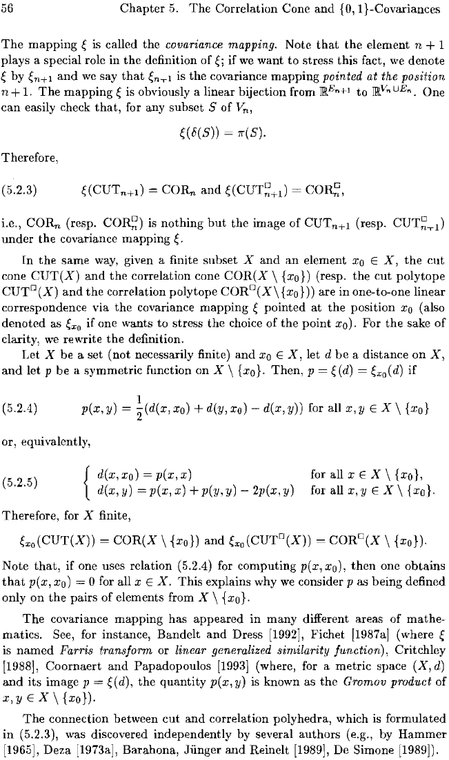
The

mapping

~

is called the covariance mapping. Note

that

the element n + 1

plays a special role in

the

definition of

~i

if

we

want to stress

this

fact,

we

denote

~

by

~n+l

and

we

say

that

~nTl

is

the

covariance mapping pointed at the position

n + 1.

The

mapping

~

is obviously a linear bijection from

]W.Bn+1

to

]W.Vn

UEn.

One

can

easily check

that,

for any subset S of V

n

,

~(8(S))

7r(S).

Therefore,

(5.2.3)

i.e.,

COR"

(resp.

COR~)

is

nothing

but

the image

of

CUTn+l (resp.

CUT~Tl)

under the covariance mapping

~.

In

the

same

way,

given a finite subset X and

an

element

Xo

EX,

the

cut

cone

CUT(X)

and

the

correlation cone

COR(X

\ {xo}) (resp. the

cut

polytope

CUTD(X)

and

the

correlation polytope

CORD(X\

{xo})) are in one-to-one linear

correspondence via

the

covariance mapping

~

pointed

at

the position

Xo

(also

denoted

as

~xo

if one wants to stress the choice of the point xo). For the sake of

clarity,

we

rewrite

the

definition.

Let

X be a set (not necessarily finite)

and

Xo

EX,

let d

be

a distance on

X,

and

let p be a symmetric function on X \ {xo}. Then, p =

~(d)

~xo(d)

if

(5.2.4)

1

p(x, y) = 2(d(x, xo) +

dey,

xo) - d(x, y)) for all x, y

EX

\ {xo}

or, equivalently,

(5.2.5)

{

d(x,xo)=p(x,x)

d(x, y) = p(x, x) + p(y, y) - 2p(x, y)

Therefore, for X finite,

for all

x E X \ {xo},

for all

x,y

EX

\ {xo}.

~xo(CUT(X))

=

COR(X

\ {xo})

and

~xo(CUTD(X))

= CORD(X \ {xo}).

Note

that,

if one uses relation (5.2.4)

for

computing p(x, xo),

then

one obtains

that

p(x, xo) 0 for all x E

X.

This explains why

we

consider p as being defined

only on

the

pairs of elements from X \ {xo}.

The

covariance mapping has appeared in many different areas of mathe-

matics. See, for instance, Bandelt

and

Dress [1992]' Fichet

[1987aJ

(where

~

is named Farris transform or linear generalized similarity function), Critchley

[1988], Coornaert and Papadopoulos

[1993]

(where,

for

a metric space (X,

d)

and

its

image p =

~(d),

the quantity

p(x,y)

is

known as

the

Gromov product of

x,yEX\{xo}).

The

connection between cut

and

correlation polyhedra, which

is

formulated

in

(5.2.3), was discovered independently by several authors (e.g., by Hammer

[1965]' Deza [1973a], Barahona, Junger

and

Reinelt

[1989],

De Simone [1989]).

5.2

The

Covariance

Mapping

57

As a consequence

of

(5.2.3), every inequality valid for

the

cut

polytope

CUT~+l

can

be

transformed

into

an

inequality which

is

valid for

the

correla-

tion

polytope

CO~

and

vice versa, via

the

covariance mapping. We

formulate

this

fact

in

a precise way in

Proposition

5.2.7 below.

"cut

side"

d E

II~En+l

6(S) (

for

S

~

V

n

)

CUTn+1

CUT~+l

Triangle

inequalities:

d(i,j)

-

d(i,n

+

1)

-

d(j,n

+ 1)::; 0

d(i,n

+ 1) -

d(j,n

+ 1) -

d(i,j)::;

0

d(j,n

+ 1) -

d(i,n

+ 1) -

d(i,j)

::;

0

d(i,n

+ 1) +

d(j,n

+ 1) +

d(i,j)::;

2

d(i,j)

- d(i, k) -

d(j,

k)

::;

0

d(i,j)

+ d(i, k) +

d(j,

k)

::;

2

Hypermetric

inequalities:

l~i<j~n+1

withbEZ

n

+1,

L b

i

=l

l~i~n+l

Negative

type

inequalities:

l~i<j~n+l

withbEZ

n

+1,

L

bi=O

l~i~n+l

L

bibjd(i,j)

::;

k(k

+ 1)

lSi<j~n+1

with

bE

zn+1,

L b

i

=

2k

+ 1

l~i~n+l

"correlation

side"

P E

m.VnUEn

7l"(S)

CORn

COR~

0::;

Pij

::; Pii

Pij

::;

Ph

Pii +

Ph

-

Pij

::; 1

-Pkk

-

Pij

+ Pik +

Pjk

::; 0

Pii +

Ph

+

PH

-

Pij

- Pik -

Pjk

::; 1

with

bE

zn

( i.e., ( L

biPi)(

L biPi - 1)

?:

0,

l<i<n l<i<n

setti~g

Pii

:=

J;;,Pij

:=

PiPj)

l:Si,j~n

with

bE

zn

( L biPi -

k)(

L biPi - k - 1)

?:

0

l:Si:Sn

l:Si'Sn

with

bE

zn,

k E Z

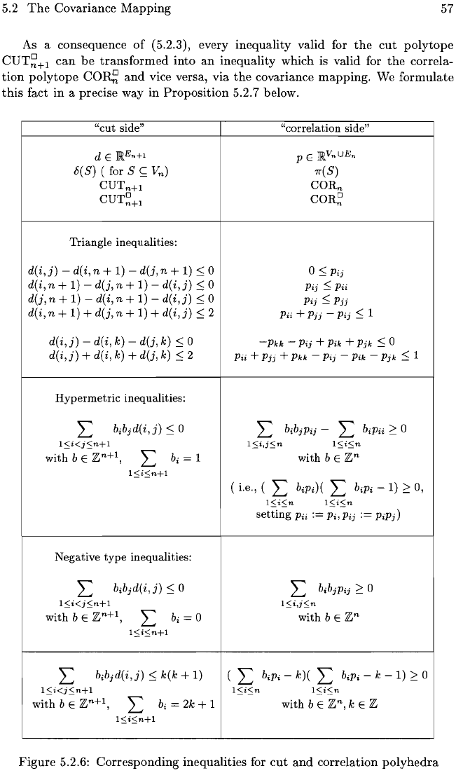
Figure

5.2.6: Corresponding inequalities for

cut

and

correlation

polyhedra

58

Chapter

5.

The

Correlation Cone

and

{O,

1 }-Covariances

We show in

Figure

5.2.6 how

this

correspondence applies

to

several classes

of

in-

equalities, namely,

to

the

triangle inequalities,

the

hypermetric

inequalities,

and

to

the

negative

type

inequalities (these inequalities will be

treated

in Section 6.1

and,

in

full detail,

in

Chapter

28).

Proposition

5.2.7.

Let

a E

~Vn,

b E

~En,

C E

~En+l

be

linked

by

{

Ci,n+l

Cij

l~j~n,

#i

=

-!bij

for 1

:s:

i

:s:

n,

for 1

:s:

i < j

:s:

n.

Given a E

~,

the inequality

l:

cijd(i,j)

:s:

a

l~i<j~n+l

is valid (resp. facet defining) for the cut polytope

CUT~+l

if

and only

if

the

inequality

l:

aiPii

+

l:

bijPij:S: a

l~i~n

l~i<j~n

is valid (resp. facet defining) for the correlation polytope

COR~.

I

5.3

Covariances

We present here several characterizations for

the

members

of

the

correlation

cone

and

polytope;

they

are

counterparts

to

the

results

of

Section 4.2, via

the

covariance

mapping.

We first introduce

the

notion

of

M-covariance.

This

notion

is

studied

in Assouad [1979, 1980b] for M being a subset

of

a

Hilbert

space. We

consider here only

the

cases

when

M =

~

or M =

{O,

I}.

Definition

5.3.1.

Let M

be

a subset

ofR

A symmetric function p : X x X

--+

~

is called an M-covariance

if

there exist a measure space (n,A,JL) and functions

f x

E

L2

(n,

A,

JL)

(for x

EX)

taking values in

M,

and such that

p(x,

y) = k

fx(w)fy

(w)JL

(dw) for all

x,

y E

X.

In particular, p is a

{O,

1 }-covariance

if

and only

if

there exist a measure space

(n,

A,

JL)

and sets

Ax

E AI' (jor x

EX)

such that

p(x,

y) =

JL(Ax

nAy)

for all

x,

y E

X.

The

shows how

~-covariances

and

{O,

1 }-covariances are

2

-

and

Ll-embeddable

distance

spaces, respectively (via

the

covariance

map-

ping).

Lemma

5.3.2.

Let X

be

a set and

Xo

E

X.

Let d

be

a distance on X and let

p

=

exo

(d)

be

the corresponding symmetric function on X \ {xo}. Then,

5.3 Covariances

59

(i)

(X,

Vd)

is

L2

-embeddable

if

and only

if

p is an

~-covariance

on X \ {xo}.

(ii)

(X,

d)

is LI -embeddable

if

and only

if

p is a

{O,

1 }-covariance on X \ {xo}.

Proof. (i) is

an

immediate

verification; (ii) too, using

Lemma

4.2.5.

I

Therefore, for X finite, p is a

{O,

1 }-covariance on X if

and

only if p belongs to

the

correlation

cone

COR(X).

The

following finitude result

is

a consequence

of

Lemma

5.3.2

and

Theorem

3.2.1.

Proposition

5.3.3.

Let

p

be

a

symmetric

function

on

X.

Then, p is a {0,1}-

covariance on X

if

and only if, for each finite subset Y

of

X,

the restriction

of

p to Y is a

{O,

1}-covariance on

Y.

I

We now give

an

interpretation

of

the

members of

the

correlation cone

and

polytope

in

terms

of

correlations of events in a measure space; it

is

the

analogue

of

Proposition

4.2.1 (via

the

covariance mapping).

It

was rediscovered in Pitowsky

[1986].

Proposition

5.3.4.

Let

p = (Pij

h<:i<:j<:n

E

~VnUEn.

The following assertions

are equivalent.

(i) p E CORn (resp. p E

COR~).

(ii) There exist a measure space (resp. a probability space)

(n,A,

/L)

and events

AI,

.

..

,An

E A such that Pij = /L(Ai n

Aj)

for

aliI

~

i

~

j

~

n.

I

As a consequence of

Proposition

5.3.4, every inequality valid for

the

correla-

tion

polytope

COR~

can

be

interpreted

as

an

inequality

that

is

satisfied by

the

joined

probabilities

of

a set

of

n events. Consider, for instance,

the

inequalities

(on

the

"correlation side") corresponding to

the

first four triangle inequalities

in

Figure

5.2.6.

They

express some very simple properties

of

joined probabilities.

The

first

three

express

the

fact

that

the

probability

/L(

Ai

n

Aj)

of

the

intersection

of

two events

Ai,

Aj

is nonnegative

and

less

than

or equal to each of

the

proba-

bilities

/L(A

i

),

/L(A

j

).

The

fourth one simply says

that

the

probability /L(Ai

UA

j

)

of

the

union

of two events

is

less

than

or equal to one.

For

the

members

of

the

correlation cone which can

be

written

as a nonneg-

ative

integer linear

combination

of

correlation vectors,

we

can assume

that

the

measure

space

in

Proposition

5.3.4 (ii) is endowed

with

the

cardinality measure.

Namely,

we

have

the

following result, which

is

an

analogue

of

Proposition

4.2.4

(i)

~

(iii) (via

the

covariance mapping).

Proposition

5.3.5.

Let p = (Pijh<:i<:j<:n E

~VnUEn.

The

following assertions

are equivalent.

(i)

P = L

>"s7I"(8)

for

some

nonnegative integers

>..s.

SS;;Vn

60

Chapter

5.

The

Correlation Cone

and

{O,

1 }-Covariances

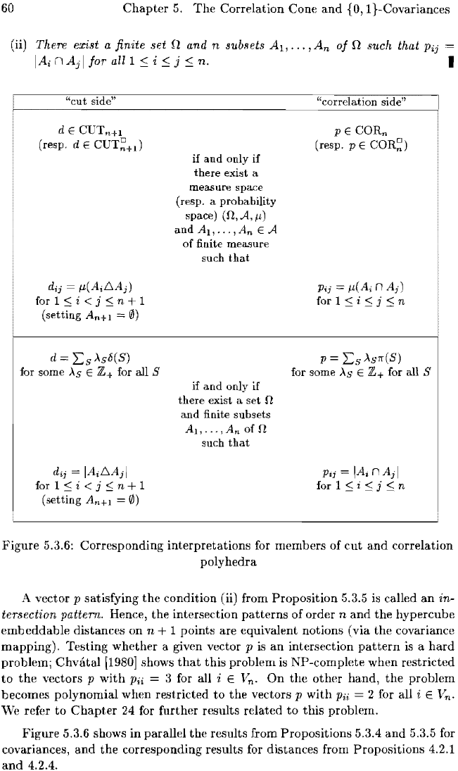
(ii) There exist a finite set

nand

n subsets

Al,

...

,An

of n such

that

Pij

IAinAjlforalll::;i::;j

n. I

dE

(resp. d

d

ij

It(

AiL',Aj)

for 1

::;

i < j

::;

n + 1

(setting

A

n

+

1

"'"

@)

d"",

LSAS8(S)

for some

AS

E Z+ for all S

dij

= IAiL',Ajl

for 1

::;

i < j

::;

n + 1

(setting

An+!

=

0)

if

and

only

if

there

exist a

measure space

(resp. a probability

space)

(n, A,

It)

and

Al,

...

,An

E A

of

finite measure

such

that

if

and

only if

there

exist a set n

and

finite subsets

Al,

...

,An

ofn

such

that

P E CORn

(resp. p E

COR~)

Pij

"'"

It(Ai

n

Aj)

for 1 ::; i

::;

j

::;

n

P =

Ls

AS1r(S)

for some

AS

E for all S

Pij

1·4i

n

for1::;i::;j

n

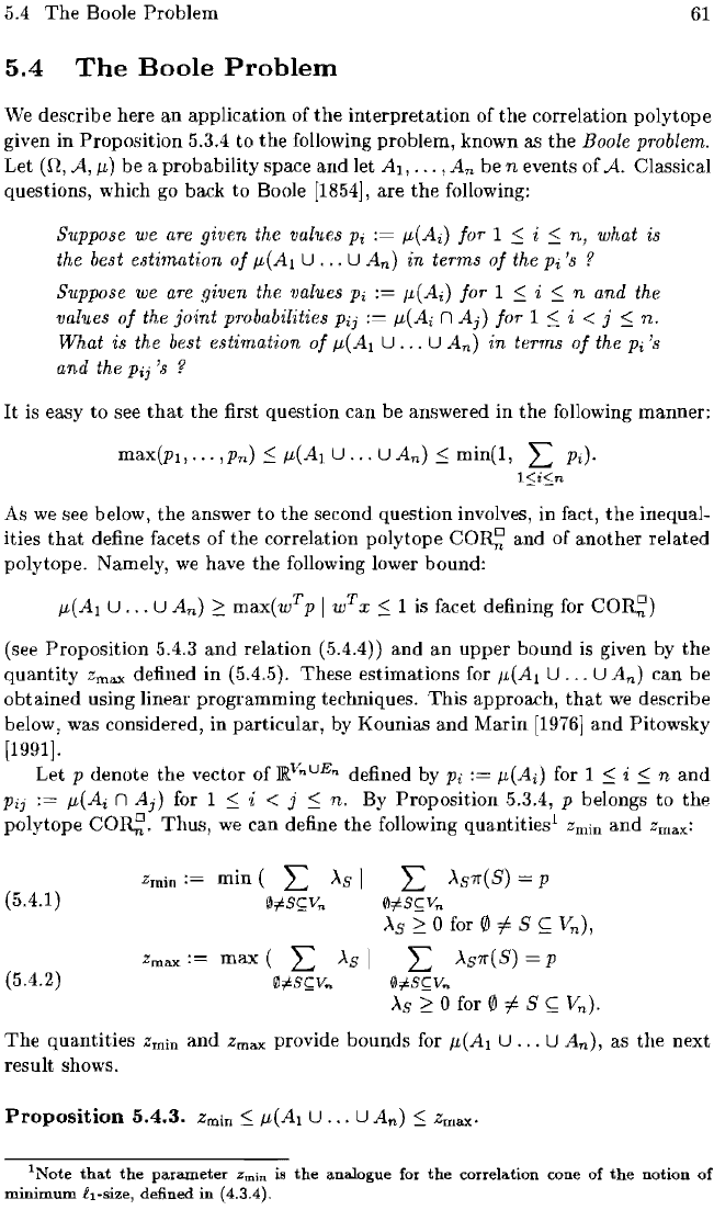
Figure 5.3.6: Corresponding interpretations

for

members of

cut

and

correlation

polyhedra

A vector

P satisfying

the

condition (ii) from Proposition 5.3.5 is called

an

in-

tersection pattern.

Hence, the intersection

patterns

of order n and the hypercube

embeddable distances on

n + 1 points are equivalent notions (via the covariance

mapping). Testing whether a given vector

P

is

an

intersection

pattern

is

a

hard

problem;

Chvatal

[1980]

shows

that

this problem is NP-complete when restricted

to

the

vectors p

with

Pi;

3 for all i E V

n

.

On

the other hand, the problem

becomes polynomial when restricted

to

the

vectors P

with

Pii

2

for

all i E V

n

.

We refer to

Chapter

24 for further results related

to

this problem.

Figure 5.3.6 shows in parallel the results from Propositions 5.3.4

and

5.3.5 for

covariances,

and

the corresponding results for distances from Propositions 4.2.1

and

4.2.4.

5.4

The

Boole

Problem

61

5.4

The

BoDle

Problem

We describe here

an

application of

the

interpretation of

the

correlation polytope

given

in

Proposition

5.3,4 to

the

following problem, known as

the

Boole problem.

Let

(n, A,

p,)

be

a probability space

and

let

...

,

An

be

n events of.A. Classical

questions, which go back

to

Boole [1854], are

the

following:

Suppose we

are

given the values Pi P,(Ai) for 1

::;

i

::;

n,

what is

the best estimation

of

P,(AI U

...

U

An)

in terms

of

the Pi'S ?

Suppose

we

are given the values Pi I.L(A;) for 1

::;

i

::;

n and the

values

of

the }oint pmbabilities

Pij

p,(Ai n

Aj)

for 1

::;

i < }

::;

n.

What is the best estimation

of

P,(AI u

...

U

An)

in terms

of

the Pi'S

and the

Pij

'13

?

It

is easy

to

see

that

the

first question

can

be

answered in

the

following manner:

As

we

see below,

the

answer

to

the

second question involves, in

the

inequal-

ities

that

define facets

of

the

correlation polytope

COR~

and

of another

we

have

the

following lower bound:

p,(Al

U

...

U

An)

2:

max(w

T

pi

w

T

X ::;

1 is facet defining for

CO~)

(see

Proposition

5.4.3

and

relation (5.4.4»

and

an

upper

bound is given by

the

quantity

Zma.x defined

in

(5.4.5). These estimations for I.L(AI U

...

U

An)

can

be

obtained

using linear programming techniques.

This

approach,

that

we

describe

below, was considered, in particular, by Kounias

and

Marin

[1976]

and

Pitowsky

[1991].

Let

P denote

the

vector of

liV"UE"

defined by Pi

:=

p,(Ai)

for 1

::;

i

::;

nand

Pij

p,(A; n

Aj)

for 1

::;

i < }

::;

n. By Proposition 5.3.4, P belongs to

the

polytope

CO~.

Thus,

we

can define

the

following quantities

l

Zmin

and

Zma.x:

Zmin

:=

min

(

L

>'s

I

L

>'S7r(S)

= P

(5.4.1)

0;B

(;:

V"

0;B<;;v"

>'s

2:

0 for 0

i=

S

~

V

n

),

Zmax

max

(

L

>'s

I

L

>'S7r(S)

= P

(5.4.2)

0iS

<;;

V"

0iS<;;v"

>'s

2:

0 for 0

i=

S

~

V

n

)·

The

quantities Zmin

and

Zmax

provide

bounds

for

IL(AI

U

...

U

An),

as

the

shows.

Proposition

5.4.3.

Zmin::;

p,(Al

U

...

U

An)

::; Zmax.

'Note

that

the

parameter

Zmin

is

the

analogue for

the

correlation cone

of

the

notion

of

minimum

il-size,

defined in (4.3.4).

Deza M.M., Laurent M. Geometry of Cuts and Metrics

Подождите немного. Документ загружается.