Deza M.M., Laurent M. Geometry of Cuts and Metrics
Подождите немного. Документ загружается.

10
Chapter
1.
Outline
of
the
Book
mension
up
to
llog2 n
J.
This
indicates
that
MET~
is
wrapped
quite
tightly
around
CUT~.
In Section 31.7,
the
Euclidean distance from
the
hyperplane
supporting
a facet
of
CUT~
to
the
barycentrum
of
CUT~
is
considered.
It
is
conjectured
that
this
distance is minimized by triangle facets.
The
conjecture
is
verified for all facets defined by
an
inequality
with
coefficients
in
{O,
1,
-I}
and
asymptotically
for some
other
cases. Simplex facets are considered
in
Sec-
tion
31.8.
It
turns
out
that
for n
::;
7
the
great
majority
of
facets of
CUT~
are
simplices.
In fact
about
97% of
the
facets of
CUT~
are
simplices!
This
may
well
be
a general
phenomenon
for any n.
Further
geometric results are presented
in
Sections 31.1-31.4.
Borsuk
[1933]
asked
whether
it is possible
to
partition
every set X
of
points
in
JRd
into d + 1
subsets,
each having a smaller
diameter
than
X.
This
question was answered
in
the
negative by
Kahn
and
Kalai [1993] by a
construction
using cuts,
that
we
present
in
Section 31.1.
The
result
in
Section 31.2 indicates how
to
obtain
valid
inequalities for pairwise angles among a set
of
vectors from
the
valid inequalities
for
the
cut
polytope.
This
permits
in
particular
to
answer
an
old question
of
Fejes
T6th
[1959] concerning
the
maximum
value for
the
sum
of
the
pairwise angles
among
a set
of
n vectors. Section 31.3 deals
with
the
completion
problem
for
partial
positive semidefinite matrices.
It
turns
out
that
necessary conditions for
this
completion
problem
can
be
obtained
from
the
valid inequalities for
the
cut
polytope,
as a reformulation of
the
result
in
Section 31.2. Finally, Section 31.4
deals
with
the
completion
problem
for
partial
Euclidean matrices;
that
is,
with
the
study
of
the
projections
of
the
negative
type
cone.
These
two
completion
problems
are closely related
and
have
intimate
links
with
the
polyhedra
under
investigation
in
this
book.
M.M. Deza, M. Laurent, Geometry of Cuts and Metrics, Algorithms and Combinatorics 15,
DOI 10.1007/978-3-642-04295-9_2, © Springer-Verlag Berlin Heidelberg 2010
Chapter
2.
Basic
Definitions
In
this
chapter
we
introduce some basic definitions
about
graphs, polyhedra, ma-
trices,
and
algorithmic complexity. We present here only
the
very basic notions;
further
definitions will
be
introduced
later
in
the
text
as
they
are needed.
The
reader
may
consult, for instance,
the
following textbooks for more detailed infor-
mation: Bondy
and
Murty
[1976]
for graphs,
Griinbaum
[1967]' Schrijver [1986]'
Ziegler
[1995]
for polyhedra, Lancaster
and
Tismenetsky
[1985]
for matrices,
and
Garey
and
Johnson
[1979]
for algorithms
and
complexity.
2.1
Graphs
A graph G = (V,
E)
consists
of
a finite
set
V
of
nodes
and
a finite set E
of
edges.
Every edge e E E consists of a
pair
of nodes u
and
v, called its endnodes;
we
then
denote
the
edge e alternatively as (u, v) or as uv. Two nodes are
said
to
be
adjacent
if
they
are joined by
an
edge. Two edges are said
to
be
parallel if
they
have
the
same
endnodes. Here,
we
will only consider simple graphs, i.e.,
graphs
in
which every edge has distinct
end
nodes
and
no two edges are parallel.
The
degree
of
a node v E V is
the
number
of edges
to
which v is incident.
When
every two nodes
in
G are adjacent,
then
the
graph
G
is
said to
be
a complete
graph.
It
is
customary
to
denote
the
complete
graph
on n nodes by Kn;
we
can
suppose
that
the
node set of
Kn
is
the
set
Vn
:=
{I,
...
,n}
and
that
its
edge set
is
the
set En
:=
{ij
I i
-I
j E V
n
} (where
the
symbol
ij
denotes
the
unordered
pair
of
the
integers
i,j,
i.e.,
ij
and
ji
are considered identical).
A
graph
G is said to
be
bipartite if
its
node set
can
be
partitioned
into
V =
VI
U V
2
in
such a way
that
no two nodes
in
VI
and
no two nodes
in
V2
are
adjacent.
The
sets VI,
V2
are said to form a bipartition
of
G.
If
G is
bipartite
with
bipartition
(VI, V
2
)
and
if every node
in
VI
is adjacent
to
every node
in
V
2
,
then
G is called a complete bipartite graph. We let K
nl
,n2
denote
the
complete
bipartite
graph
with
bipartition
(VI, V
2
) where
JVII
=
ni
and
JV21
=
n2.
The
complete
bipartite
graph
KI,n
(n:2:
1)
is sometimes called a star.
Given a node subset S
<:::;
V
in
a
graph
G, let oG(S) denote
the
set
of
edges
in
G having one endnode
in
S
and
the
other
endnode
in
V \
S;
oG(S)
is
called
the
cut
I determined by
S.
'Thus,
the
symbol
tia(S)
denotes
here
an
edge
set.
In
fact,
the
symbol
ti(S) will
be
mostly
used
in
the
book
for
denoting
a 0-1
vector,
namely,
the
cut
semimetric
determined
by
S (see
Section
3.1).
When
G is
the
complete
graph
K
n
,
then
the
incidence
vector
of
the
cut
tia(S)
12
Chapter
2.
Basic Definitions
Let
G = (V,
E)
be a graph. A
graph
H = (W,
F)
is
said
to
be a subgraph
of
G
if
W
S;;
V
and
F
S;;
E. Given a node subset W
S;;
V,
G[W] denotes
the
subgraph
of G induced by
W;
its node set is
Wand
its
edge
set
consists of
the
edges
of
G
that
are contained in
W.
The
set W
is
said
to
induce a clique
in
G if
any
two nodes
in
Ware
adjacent, i.e., if G[W]
is
a complete
graph.
A
matching
in
G is
an
edge
subset
F
S;;
E such
that
no two edges in F
share
a
common
node; a
matching
F is a perfect matching if every node of G belongs
to
exactly
one edge
in
F.
Given
an
edge
subset
F
S;;
E
in
G,
G\F
:=
(V, E \
F)
is called
the
graph
obtained
from G by deleting
F.
When
F = {e}
we
also denote
G\
{e} by
G\e.
Contracting
an
edge e
:=
uv
in
G
means
identifying
the
endnodes u
and
v
of
e
and
deleting
the
parallel edges
that
may
be
created
while identifying u
and
v;
G/e
denotes
the
graph
obtained
from G by contracting
the
edge
e.
For
an
edge
set
F
S;;
E,
G / F denotes
the
graph
obtained
from G by contracting all edges of
F (in any order). A
graph
H is said to be a
minor
of G
if
it
can be
obtained
from G by a sequence
of
deletions
and/or
contractions of edges,
and
deletions
of
nodes.
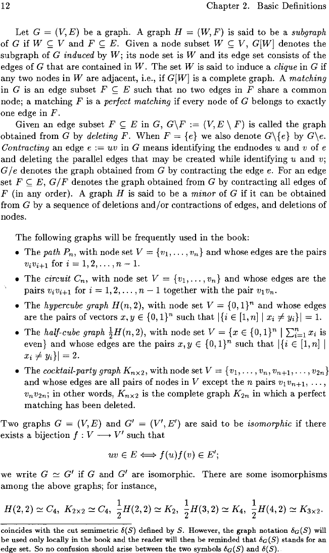
The
following
graphs
will be frequently used in
the
book:
•
The
path P
n
,
with
node set V =
{VI,
...
, v
n
}
and
whose edges are
the
pairs
ViVi+1
for i =
1,2,
...
,n
-
l.
•
The
circuit
en,
with
node set V =
{VI"'"
v
n
}
and
whose edges are
the
pairs
ViVi+1
for i =
1,2,
...
,n
- 1 together
with
the
pair
VI V
n
.
•
The
hypercube graph
H(n,
2),
with
node set V = {O,l}n
and
whose edges
are
the
pairs
of vectors
x,
Y E {a, l}n such
that
I
{i
E
[1,
n]1
Xi
i=
Yi}
I =
l.
•
The
half-cube graph
!H(n,2),
with
node set V =
{x
E {O,l}n I
L~IXi
is
even}
and
whose edges are
the
pairs
X,Y
E
{o,l}n
such
that
I{i
E [l,n] I
Xi
i=
Yi}1
= 2.
•
The
cocktail-party graph
Knx2'
with
node set V =
{VI,
...
, V
n
,
Vn+I,.··,
V2n}
and
whose edges are all pairs of nodes in V except
the
n pairs VI V
n
+l,
...
,
VnV2n;
in
other
words,
Knx2
is
the
complete
graph
K2n
in
which a perfect
matching
has
been
deleted.
Two
graphs
G = (V,
E)
and
G' =
(V',
E')
are said
to
be
isomorphic if
there
exists a bijection f : V
--t
V'
such
that
uv
E E
~
f(u)f(v)
E E';
we
write G
~
G'
if G
and
G'
are isomorphic.
There
are some isomorphisms
among
the
above graphs; for instance,
coincides
with
the
cut
semimetric
8(S) defined
by
S.
However,
the
graph
notation
8a(S) will
be
used
only
locally
in
the
book
and
the
reader
will
then
be
reminded
that
8a(S)
stands
for
an
edge
set.
So
no
confusion
should
arise
between
the
two
symbols
8a(S)
and
8(S).

2.1
Graphs
13
The
graphs C5,
H(3,2)
and
K3X2
are depicted in Figure 2.1.1.
The
Petersen
graph P
lO
,
which will also be used on several occasions, is shown in Figure 2.1.2.
o
circuit C 5
hypercube graph H(3,2)
cocktail-party graph K 3x2
Figure 2.1.1
Figure 2.1.2:
The
Petersen graph
PlO
A
graph
G is said
to
be connected
if,
for every two nodes
u,
v
in
G, there
exists a
path
in G joining u
and
Vi
a graph which is not connected is said
to
be
disconnected. A forest is a
graph
which contains no circuit; a tree is a connected
forest. A
cycle or Eulerian graph is a
graph
which
can
be decomposed as
an
edge
disjoint union
of
circuits (equivalently,
it
is a graph
in
which every node has
an
even degree).
Let us now consider two operations
on
graphs:
the
Cartesian product and
the
clique
sum
operation. Let G
I
= (VI,E
I
)
and
G2
=
(V
2
,E
2
)
be two graphs.
Their
Cartesian product G
I
X G
z
is the graph G
:=
(VI X V
2
,
E)
with node set
and
whose edges are
the
pairs
((UI'
U2),
(VI,
V2))
(with
ul,
VI
E
VI
and
U2,
V2
E
V2)
such
that,
either
(uI,vd
E and
U2
V2,
or
UI
VI
and
(U2,V2)
E E
2
·
Let G = (V,
E)
be a graph. Let
VI
and
V
2
be subsets of V such
that
V =
VI U
V2
and
such
that
the
set W
:=
Vi
n
V2
induces a clique in G. Suppose
moreover
that
there is no edge joining a node in
VI
\ W to a node in
V2
\
W.
Then,
G is called
the
clique
k-sum
of the graphs
Gl
:=
G[Vl]
and
G2
:=
G[V2],
where k
:=
IWI.
One may say simply
that
G is
the
clique
sum
of G
l
and
G
2
if
one does
not
wish to specify the size of the common clique.
14
Chapter
2.
Basic Definitions
For a
graph
G, its suspension graph
VG
denotes the
graph
obtained
from G
by
adding a new node (called
the
apex
of
VG)
and
making
it
adjacent
to
all
the
nodes
in
G. Moreover,
the
line graph
of
G is
the
graph
L(G)
whose nodes are
the
edges
of
G
with
two edges adjacent
in
L( G)
if
they
share
a common node,
2.2
Polyhedra
We
assume familiarity
with
basic linear algebra.
By
jR
(resp.
Q,
Z,
N)
we
mean
the
set
of
real (resp, rational, integer,
natural)
numbers. Given a set E
and
a
subset
S
~
E,
the
incidence vector
of
S is
the
vector X
S
E
JRE
defined by
X
s
.=
{ 1
e . 0
if
e E S,
if
e E E \ S.
If
A
and
B are subsets of E,
then
A6B
denotes
their
,~ymmetric
difference
defined by
A6B
= (A U
B)
\ (A n
B).
For a
matrix
M,
we
let
MT
denote its transpose
matrix;
similarly, x
T
denotes
the
transpose of a vector x. Hence,
n
x
T
y =
L:
XiYi
for x, Y E
lIRn.
·;=1
We
remind
that
the
dimension
of
a set X
~
lR'"
is defined as
the
cardinality
of
a
largest affinely independent subset
of
X minus one; it is denoted as
dim(X).
The
set X
~
jRn is said
to
be
full-dimensional if
dim(X)
= n.
The
rank of
X,
denoted
as
rank(X),
is defined as
the
cardinality
of
a largest linearly independent
subset
of
X.
Let
us introduce some
notation
for linear hulls. Given a set X
~
jRn
and
K
~
lR,
set
K(X)
:=
{L:
AxX
I
Ax
E K for all x
EX}.
xEX
(In
this
definition
we
suppose
that
only finitely
many
Ax'S are nonzero.)
When
K
Z,
the
set
Z(X)
is called
the
integer hull of
X;
when K
114,
the set
(X)
is
called
the
conic hull
of
X;
when K =
Z+,
the
set
Z+(X)
is known as
the
integer cone generated
by
X.
We
will also consider the affine integer hull of
X,
defined as
{
L:
AxX
I
Ax
E Z for all x E X
and
L:
Ax
1 }
~X
xEX
and
the convex hull
of
X,
defined as
Conv(X)
{L:
Ax
X
I
Ax
:::>:
0 for all x E X
and
L:
Ax
= I}.
xEX
xEX
A
set
X
~
jRn
is
said
to
be
convex if
Conv(X)
=
X.
A convex
body
in
jRn is
a convex subset of
jRn which
is
compact
and
full-dimensional.
The
polar
XO
of
X
~
jRn
is
defined as
2.2
Polyhedra
15
The
set X is said
to
be
centrally
symmetric
if
-x
E X for all x E
X.
We now
consider
in
detail conic
and
convex hulls.
Cones
and
Polytopes.
We
recall here several basic definitions concerning
cones
and
polytopes. Given a subset X
<;;;;
TIRn,
the
set X is said
to
be a cone
2
if
1I4
(X)
=
X.
If
C is a cone
of
the
form C
(X),
one says
that
C is generated
by X
and
the
members
of
X are called its generators.
The
cone C is said
to
be
finitely generated
if
it
admits
a finite set of generators, i.e.,
if
C =
1I4
(X)
for
SOme
finite set
X.
The
polar
of a cone C
]Rn
can alternatively
be
described as
co
=
{x
E
]Rn
I x
T
y
:s:
0 Vy E C.}
Every convex set
of
the
form Conv(X), where X is finite,
is
called a polytope.
Let A
be
an
m x n
matrix
and
let b E
]Rm
be
a vector.
Then,
the
set
is called a polyhedron. Every polyhedron is obviously a convex set
and
it
is a
cone when b is
the
zero vector. Every cone of
the
form
{x
E
]Rn
I
~4x
:s:
O}
is
called a
polyhedral cone.
A classical result, generally
attributed
to
Minkowski
and
Weyl, asserts
that
polytopes
and
bounded
polyhedra are, in fact,
the
same notions. (A set P E
]Rn
is
said
to
be bounded
if
there exists a constant R such
that
IXil
:S:
R
for all x =
(Xi)~l
E P.)
In
other
words, every polytope
P,
is given as
the
convex hull of a finite
set
X,
can
be
expressed as
the
solution set
of
a finite
system
Ax
:S:
b of linear inequalities; such a system is called a linear description
of
P.
The
converse
statement
holds as well.
There
is a similar result for cones:
A cone C is finitely generated
if
and
only
if
it
can
be
expressed as
the
solution
set
of
a system
Ax
:S:
0
of
linear inequalities; such a system is called a linear
description
of
C.
In
other
words, a cone is finitely generated
if
and
only
if
it
is
polyhedral.
In
practice, finding a linear description
of
a polytope P or of a cone C (as-
suming
that
they
are by
their
generators) may
be
a
hard
task. One of
our
main
objectives
in
this book will be,
in
fact,
to
give information
about
the
linear
description
of
a specific polytope
and
cone, namely,
the
cut
polytope
and
the
cut
cone:
CUT~
Another
well-known result
that
we
will sometimes apply is CaratModory's
theorem,
which
can
be
stated
as follows: Let X
<;;;;
]Rn.
If
x E
lI4(X)
then
x E
lI4(X'),
where
X,
is a linearly independent subset
of
X.
If
x E
Conv(X)
then
x E
Conv(X'),
where
X'
is
an
affinely independent subset
of
X.
The
folJlowing
polytopes will
be
frequently llsed in
the
book:
in
this
definition a cone is always
assumed
to
be
convex.
16
Chapter
2.
Basic Definitions
•
The
n-dimensional simplex an; this
is
the polytope
n
Conv(O,el,
...
,en)={xE]RnIO
Xi
1
(l:S;i:S;n),Lx;:S;l}.
i=l
•
The
n-dimensional cross-polytope
!3n;
this is the polytope
n
aiXi:S;
1 for all a E
{±l}n}.
•
The
n-dimensional hypercube
')'n;
this
is
the polytope
Conv({O,l}n)
[o,l]n.
(Here, e1,
...
,
en
denote the coordinate vectors
in
]Rn.)
Two polytopes
P,
pI
in
]Rn are said to be affinely equivalent if
pI
=
f(P),
where f is
an
affine bijection
of
]Rn.
A simplex
is
any polytope of
the
form
Conv(X),
where
the
set X is affinely
independent. Similarly, a
simplex cone is a cone of
the
form
(X),
where the
set
X is linearly independent.
We
use, in fact, the symbol O:n for denoting any
n-dimensional simplex. Similarly,
,en
and ')'n denote
the
above cross-polytope
and
hypercube,
up
to affine bijection.
~ote
that
aI,
!31
and
')'1 coincide,
and
that
!32
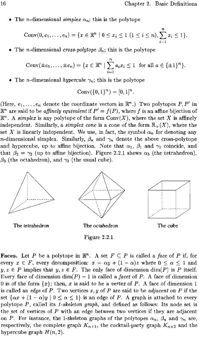
= ')'2 (up to affine bijection). Figure 2.2.1 shows 0:3 (the tetrahedron),
!33 (the octahedron),
and
~f3
(the usual cube).
The tetrahedron The octahedron
The cube
Figure 2.2.1
Faces.
Let P
be
a polytope in ]Rn. A set F
~
P is called a face
of
P
if,
for
every
x E every decomposition: x
o:y
+
(1
-
a)z
where 0
:S;
a
:S;
1 and
y, z E P implies
that
y, z E
F.
The
only face of dimension
dim(P)
is
P itself.
Every face of dimension
dim(P)
1 is called a facet of
P.
A face of dimension
o is of
the
form
{x};
then, x is said
to
be
a vertex of
P.
A face
of
dimension 1
is called
an
edge of
P.
Two vertices
x,
y of P are said to
be
adjacent on P if
the
set
{O:x
+
(1
a)y
lOa
:S;
I}
is
an
edge of P. A graph
is
attached to every
polytope
P,
called
its
i-skeleton
graph, and defined as follows: Its node set is
the
set of vertices of P with an edge between two vertices if they are adjacent
on
P. For instance,
the
I-skeleton graphs of the polytopes
O:n,
!3n
and
')'n
are,
respectively,
the
complete graph K
n
+
b
the cocktail-party graph
Knx2
and
the
hypercube
graph
H(n,
2).
2.2
Polyhedra
17
A face F of P is called a simplex face if F is a simplex, i.e., if
the
vertices of
P lying
on
Fare
affinely independent.
Given a vector
v E
JRn
and
Va
E
JR,
the
inequality v
T
x
::::
Va
is
said
to
be valid
for P
if
v
T
x
::::
Va
holds for all x E P.
Then,
the
set
F : = {x E P I v
T
X
=
va}
is clearly a face of
P;
it
is called
the
face induced by
the
inequality v
T
x
::::
Va.
In
fact, every face of P is
induced
by some valid inequality.
The
above definitions
extend
to
cones
in
the
following
way.
Let C be a cone
in
JR
n
.
A face
of
C is
any
subset
F
<;
C such
that,
for every x E
F,
every
decomposition:
x = y + z where y, z E C implies
that
y, z E
F.
A face
of
dimension
dim(
C)
- 1 is called a facet
of
C; a face
of
dimension 1 is called
an
extreme
ray of
C.
Given V E
JR
n
,
the
inequality v
T
x::::
0 is said to be valid for C
if v
T
x:::: 0 holds for all x E
C.
Then,
the
set
{x
E C I v
T
X
= o}
is called
the
face
of
C induced by
the
valid inequality v
T
x
::::
o.
When
C
is
a
polyhedral
cone, every face of C arises in
this
manner.
A face F of a cone C
is
called a
simplex
face if F
is
a simplex cone.
Linear
Programming
Duality.
A linear programming problem consists of
maximizing
(or minimizing) a linear function over a polyhedron. A typical ex-
ample
of
such a
problem
is:
(P)
also
written
as
max
cTx
s.t. Ax:::: b
where A is
an
m x n
matrix,
b E
JRm
and
c E
JRn.
The
linear function c
T
x
is
often called
the
objective
function
of
the
program
(P). To
the
linear
program
(P)
is associated
another
linear
program
(D), called its dual
and
defined as
(D)
min(b
T
y
I
yT
A = c
T
, Y ?
0).
One
refers to
(P)
as
to
the
primal
program.
The
following result, known as
the
linear programming duality theorem, establishes a
fundamental
connection
between
the
linear programs (P)
and
(D).
Theorem
2.2.2.
Given an m x n
matrix
A
and
vectors b E
JR
m
,
c E
JR
n
,
then
max(
c
T
x I
Ax
::::
b)
= min( b
T
y I
yT
A = c
T
, Y ?
0)
provided both sets
{x
I
Ax
::::
b}
and
{y
I
yT
A = c
T
, Y ?
O}
are
nonempty.
I
This
theorem
admits
several
other
equivalent formulations. For example,
max(cTx
I Ax::::
b,x?
0)
=
min(bTy
I
yT
A?
cT,y?
0),
max(cTx
I
Ax
=
b,x?
0)
=
min(bTy
I
yT
A?
c
T
).
18
Chapter
2.
Basic Definitions
2.3
Algorithms
and
Complexity
Although
complexity
is
not
a central topic in this book,
we
will encounter a
number
of problems for which one
is
interested in
their
complexity
status.
We
will
not
define in a precise
mathematical
way
the
notions of algorithms
and
complexity. We only give here some 'naive' definitions, which should be sufficient
for
our
purpose. Precise definitions can be found, e.g.,
in
the
textbooks
by
Garey
and
Johnson
[1979], or
Papadimitriou
and
Steiglitz [1982].
Let
(P)
be a
problem
and
suppose, for convenience,
that
(P)
is
a decision
problem
(that
is, a
problem
which asks for a 'yes' or
'no'
answer).
We
may
take,
for instance, for (P) any of
the
following problems:
(PI)
The
i1-embeddability
problem.
Instance: A
rational
valued distance d
on
a set
Vn
=
{I,
...
,n}.
Question: Is d isometrically
iI-embeddable?
That
is, do
there
exist vectors
VI,
...
,
Vn
E qn (for some m
2:
1) such
that
d(i,j)
=
dCl
(Vi,
v
J
)
for all
i,j
E
Vn
?
(P2)
The
hypercube
embeddability
problem
for
graphs.
Instance: A
graph
G = (V,
E).
Question:
Can
G be isometrically
embedded
into some
hypercube?
An
instance
of
a problem
is
specified by providing a
certain
input.
(For
(PI),
the
input
consists of
the
G)
numbers
d(
i,
j)
while, for (P2),
the
input
consists
of
a
graph
G which can, for instance, be described by its adjacency
matrix.)
The
size of
an
instance is
the
number
of
bits
needed to represent
the
input
data
in
binary
encoding. (For instance,
the
size of
an
integer p is size(p) =
rlog2
(Ipl
+
l)l;
the
size of a
rational
number
~
is
size(p) + size(
q)
+
1;
the
size
of
an
m x n
rational
matrix
A
is
mn
+ L:i,j size(aij), etc.) Suppose
that
we
have
an
algorithm
for solving
(P).
Its
complexity is measured by counting
the
total
number
of
elementary
steps
needed to be performed
throughout
the
execution
of
the
algorithm
(elementary steps such as
arithmetic
operations, comparisons,
branching instructions, etc., are supposed to take a
unit
time).
The
algorithm
is
said to have a polynomial running time if
the
total
number
of elementary steps
can
be
expressed as p(l), where p(.)
is
a polynomial function
and
I is
the
size of
the
instance.
Problems
are classified into several complexity classes.
The
class P consists
of
the
decision problems which can be solved in polynomial time.
The
class
NP
consists of
the
decision problems for which every 'yes' answer
admits
a certificate
that
can
be checked in polynomial
time
(but
one does
not
need to know how to
find such a certificate
in
polynomial time). Similarly, a
problem
is
in co-NP if
every
'no'
answer
admits
a certificate
that
can
be checked
in
polynomial time.
Hence, P
S;;
NP
n co-NP.
For example,
the
problem
(PI)
belongs to
NP
(because
it
can be shown
that,
if d is
iI-embeddable,
then
there
exists a
set
of vectors
VI,
.
..
,V
n
E
lW.(;)
providing
an
iI-embedding
of d
and
such
that
the
size of
the
vi's is polynomially
bounded
by
that
of
d;
see Section 4.4).
On
the
other
hand,
as
we
will see
in
Chapter
19,
the
problem (P2) belongs to P.
2.4 Matrices
19
Among
the
problems in NP, some can
be
shown to be
hardest.
A
problem
is
said
to
be
NP-complete
if it belongs
to
NP
and
if a polynomial
algorithm
for solving it could be used once as a
subroutine
to
obtain
a polynomial algo-
rithm
for any problem in NP. A problem
is
NP-hard if any polynomially
bounded
algorithm
for solving it would imply a polynomial
algorithm
for solving
an
ar-
bitrary
NP-problemj note
that
the
problem itself is
not
required to be in
NP
and
that
one
permits
more
than
one call to
the
subroutine. A typical way to
show
that
a
problem
(P)
is
NP-hard
is
to
show
that
some known
NP-complete
problem
polynomially reduces to it. Given two problems (P)
and
(Q) one says
that
(Q) reduces polynomially
to
(P) if a polynomial
algorithm
solving (Q)
can
be
constructed
from a polynomial
algorithm
solving
(P).
For example,
the
hy-
percube
embeddability
problem
for
arbitrary
distances
is
NP-hard.
Typically,
the
optimization
versions
of
NP-complete decision problems are also
NP-hard.
For instance,
the
max-cut
problem:
Given W E
~n,
find a
set
S
<;;;
Vn
for
which w
T
I5(S)
is
maximum
is
NP-hard,
because
the
following problem
is
NP-complete:
Given W E
~n
and
K E Q, does there exist S
<;;;
Vn
such
that
wTI5(S)
~
K ?
(See Section 4.4.)
We
remind
that,
for two functions
f(n)
and
g(n)
(n
EN),
the
notation:
f(n)
=
O(g(n))
means
that
there
exists a
constant
C > 0
such
that
f(n)
::;
Cg(n)
for all n E
N.
Similarly,
the
notation:
f(n)
=
Q(g(n))
means
that
f(n)
~
Cg(n)
for all n E
N,
for some
constant
C >
O.
2.4
Matrices
We
group
here some preliminaries
about
matrices. A square
matrix
A
is
said to
be
orthogonal if
AT
A =
I,
i.e., if its inverse
matrix
A-l
is
equal to its
transpose
matrix
AT.
We let
OA(n)
denote
the
set
of
orthogonal n x n matrices.
The
orthogonal
matrices are
the
isometries
of
the
Euclidean spacej
that
is,
the
linear
transformations
of
lFI.
n
preserving
the
Euclidean distance. A well-known basic
fact
is
that
any two congruent sets
of
points
can be
matched
by some orthogonal
transformation.
We formulate below
this
fact for
further
reference. Recall
that
II
x
112=
VxTx
for x E
lFI.
n
.
Lemma
2.4.1.
Let
ul,
..
'
,up
E
lFI.
n
and
Vl,
•..
,vp
E
lFI.
n
be
two sets
of
vectors
such
that
II
Ui
-
Uj
112=11
Vi
-
Vj
112
for
all
i,j
= 1,
...
,po
Then, there exists
A E
OA(n)
such
that
AUi =
Vi
for
i =
1,
...
,p.
Moreover, such a
matrix
A is
unique
if
the
set
{Ul'
...
, up} has affine rank n +
1.
I
Let A = (aij)7,j=l
be
an
n x n
symmetric
matrix.
Then,
A is
said
to be
positive semidefinite if x
T
Ax
~
0 holds for all x E
lFI.
n
(or, equivalently, for all