De Felice F., Bini D. Classical Measurements in Curved Space-Times

Подождите немного. Документ загружается.

4.2 Null frames 73

Fermi-Walker transport along the null world line

Exactly as in the case of a time-like curve, one may retain only the torsion part of

the connection matrix while absorbing the curvature part into the derivative to

deﬁne a corresponding generalized Fermi-Walker transport along the null world

line, as follows:

(fw)

dλ

− C

=0. (4.80)

The world function

Spatial and temporal intervals between any two points in space-time are

physically meaningful only if their measurement is made along a curve which

joins them. A curve is a natural bridge which allows one to connect the algebraic

structures at diﬀerent points; therefore it is an essential tool to any measure-

ment procedure. The mathematical quantities which glue together the concepts of

points and curves are the two-point functions.

The most important of these is the

world function, ﬁrst introduced by Ruse (1931) and then used by Synge (1960).

As Synge himself realized, the world function is well deﬁned only locally; how-

ever, a global generalization has recently been found by Cardin and Marigonda

(2004), opening the way to a better understanding of its potential in the theory

of relativity. In de Felice and Clarke (1990) the world function was exploited to

deﬁne spatial and temporal separations between points, and to ﬁnd curvature

eﬀects in the measurement of angles and of relative velocities. Following their

work we shall recall the main properties and applications of a world function,

starting from its very deﬁnition.

Consider a smooth curve γ, parameterized by s ∈. Let ˙γ be the ﬁeld of

vectors tangent to γ. The quantity

L =

|˙γ · ˙γ|

ds (5.1)

does not depend on the parameter s and therefore it provides the seed for a

measurement of length on the curve. Given two points

and P

in the manifold,

there exist an inﬁnite number of smooth curves γ joining them. Hence, setting

= γ(s

)andP

= γ(s

), the quantity

L(s

; γ)=

|˙γ · ˙γ|

ds (5.2)

One should say many-point functions in general but we shall only consider two- and

three-point functions.

5.1 The connector 75

is a path-dependent function of the two points; clearly it vanishes if the curve is

null. We use the term world function for the quantity

Ω(s

; γ)=

, (5.3)

which is a real two-point function.

The world function is not a map between tensor ﬁelds at diﬀerent points;

therefore meaningful applications require a transport law along any given curve.

5.1 The connector

Transport laws underlie the diﬀerential operations on the manifold; examples of

these are the Lie and absolute derivatives. For the purpose of our analysis we need

to discuss in some detail the transport law which leads to the absolute derivative.

Given a curve γ with parameter s and two points on it,

= γ(s

)andP

γ(s

), we use the term connector on γ for a map

Γ(s

; γ):T

(M) → T

(M) (5.4)

which carries vectors from

to P

. The eﬀect of this map is described as

Γ(s

; γ)u

(0)

=ˇu

(1)

(5.5)

for any u

∈ T

(M) and with ˇu

∈ T

(M). Following de Felice and Clarke

(1990), we summarize the main properties of this map. The connector is subject

to the following conditions:

(i) Linearity. We require Γ to be a linear map, i.e. for any set of real numbers

and vectors u

(A)

at P

,wehave

Γ(s

; γ)(c

(A)

)=c

Γ(s

; γ)u

(A)

. (5.6)

(ii) Consistency.Ifγ joins

= γ(s

)toP

= γ(s

)andγ



joins P

= γ



)to

= γ



) then

Γ(s

; γ



)Γ(s

; γ)=Γ(s

; γ ◦ γ



), (5.7)

where the symbol ◦ means the concatenation of the curves. Hence the eﬀect

of carrying a vector from

to P

along γ and then from P

to P

along γ



is equivalent to carrying that vector from P

to P

along the curve γ ◦ γ



(iii) Parameterization independence. The result of the action of Γ along a given

curve does not depend on its parameterization.

(iv) Diﬀerentiability. We require that the result of the application of Γ(s

; γ)

varies smoothly if we vary the points

and P

and deform the whole path

between them.

The consequences of the above conditions allow one to describe the connector as

a tensor-like two-point function. Let {e

} be a ﬁeld of bases on some open set of

76 The world function

the manifold containing the pair of points and the curve connecting them. From

linearity we have

Γ(s

; γ)u

(0)

= u

Γ(s

; γ)e

= u

Γ(s

; γ)

=ˇu

, (5.8)

where the indices with subscripts 0 and 1 refer to quantities deﬁned at the points

and P

respectively. From the property of a basis we have

ˇu

= u

Γ(s

; γ)

, (5.9)

where the coeﬃcients Γ(s

; γ)

are the components of the connector. We

shall adopt the convention that the ﬁrst index refers to the tangent basis at the

ﬁrst end-point of Γ and the second index to the tangent basis at the second

end-point. From the above relation it follows that

Γ(s

; γ)

= δ

. (5.10)

The requirement of consistency by concatenation implies that

Γ(s

; γ)

Γ(s

; γ)

=Γ(s

; γ)

. (5.11)

Finally the requirement of diﬀerentiability, coupled with all the other properties

of the connector, leads to the following law of diﬀerentiation (see de Felice and

Clarke, 1990, for details):

Γ(s

,s; γ)

= −Γ(s

,s; γ)

μν

(s)˙γ

(s), (5.12)

with the initial condition given by (5.10). Here Γ

μν

are the connection coeﬃ-

cients on the manifold; they only depend on the point and not on the curves

crossing it. It is well established that the connection coeﬃcients are not the com-

ponents of a





-tensor; nevertheless they behave as the components of such a

tensor under linear coordinate transformations. This follows from the transfor-

mation properties of the components of the connector Γ(s

; γ)

; the latter

behave as a co-vector at

and as a vector at P

.From(5.9) and with respect

to a general coordinate transformation x



(x)wehave



; γ)

∂x

α

Γ(s

; γ)

∂x

β

∂x

. (5.13)

Hence from (5.12) it follows that

λ

μν



∂x

λ

∂x

μ

∂x

ν

βγ

(x) −

∂x

λ

∂x

∂

∂x

μ

∂x

ν

. (5.14)

A basic property of space-time geometry is the compatibility of the connection

with the metric, expressed by the identity

∇

μν

≡ 0. (5.15)

5.2 Mathematical properties of the world function 77

This relation stems from the requirement that the connector preserves the scalar

product. Along any curve connecting points

and P

we have

(u ·v)

=(ˇu · ˇv)

, (5.16)

with u, v ∈ T

(M) and ˇu, ˇv ∈ T

(M).

Let us conclude this brief summary by recalling the concept of geodesic on the

manifold. A curve γ connecting

to P

is geodesic if

Γ(s

; γ)˙γ

(0)

= f(s

)˙γ

(1)

, (5.17)

where f(s) is a diﬀerentiable function on γ. As stated, a geodesic can always be

reparameterized with s



(s) so that f(s



(s)) = 1; in this case the parameter s



termed aﬃne. An aﬃne parameter is deﬁned up to linear transformations.

5.2 Mathematical properties of the world function

The world function behaves as a scalar at each of its end-points and can be

diﬀerentiated at each of them separately; in this case it generates new functions

which may behave as a scalar at one point and a vector or 1-form at the other,

or as a 1-form at the ﬁrst point and as a vector at the other, and so on. To

deﬁne the derivatives of a world function we shall consider only those whose end-

points are connected by a geodesic. If we further restrict our analysis to normal

neighborhoods then the geodesic connecting any two points is unique. The world

function can be written as

Ω(s

;Υ)=

− s

)

X · X, (5.18)

where X =

Υ denotes the tangent vector to the unique geodesic Υ joining

to P

and parameterized by s. We shall now deduce the derivatives of Ω with respect to

variations of its two end-points. Let

and P

belong to smooth curves ˜γ

and ˜γ

parameterized by t,andletΥ

≡ Υ

˜γ

(t)→˜γ

(t)

be the geodesic connecting points

of ˜γ

to points of ˜γ

. We then require that the curve connecting the points P

and P

as they vary independently on the curves ˜γ

and ˜γ

is the unique geodesic

→P

. In this case the points we are considering belong also to the geodesic

so they can be referred to as P

=Υ

)andP

=Υ

). This situation

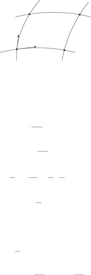
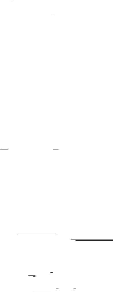
is depicted in Fig. (5.1). We then have a one-parameter family of geodesics C

with connecting vector Y =

˜γ, namely £

Y = 0. By deﬁnition we have

=0,

. (5.19)

To pursue our task let us write

Ω(Υ

), Υ

); Υ

∂Ω

∂x

∂Ω

∂x

=(s

− s

)



· X



, (5.20)

78 The world function

= γ

(t + δt)

′

∼

δt

(t)

= γ

(t + δt)

′

∼

= γ

(t)

∼

= γ

(t)

∼

(t)

∼

Fig. 5.1. The points P

=˜γ

(t)andP

=˜γ

(t) vary on the curves ˜γ

and ˜γ

and remain connected by the unique geodesic Υ

˜γ

(t)→˜γ

(t)

. The parameter on

the geodesic Υ

is s with tangent vector X while that on the curves ˜γ

and ˜γ

is t with tangent vector Y .

where {x

= x

)} and {x

= x

)} are the local coordinates for Υ

)

and Υ

) respectively. From the equation for geodesic deviation,

= R(X, Y )X, (5.21)

we deduce identically that

· X ≡ 0. (5.22)

From (5.19)

we then have



X ·





(X · Y )



=0, (5.23)

which implies that

(X · Y )=κ, (5.24)

where κ is a constant along Υ

(s). Integration along Υ

(s)froms

to s

yields

κ(s

− s

)=[X ·Y ]

; (5.25)

hence we can write (5.24) more conveniently as

(X · Y )=(s

− s

)

−1

[X ·Y ]

. (5.26)

Setting

∂Ω

∂x

, Ω

∂Ω

∂x

, (5.27)

5.2 Mathematical properties of the world function 79

and recalling (5.19)

,Eq.(5.20) becomes

dΩ

=Ω

+Ω

=(s

− s

)



· X



=(s

− s

)[X

− X

] ; (5.28)

thus

= −(s

− s

, Ω

=(s

− s

. (5.29)

From the latter we have

=Ω

=(s

− s

)

X · X =2Ω, (5.30)

or equivalently

= g

=2Ω. (5.31)

The quantities in (5.29) are the components of 1-forms deﬁned respectively at

) and Υ

). Hence diﬀerentiating one of them, say Ω



), with respect to

t, we obtain



DΩ



(0)



=Ω

+Ω

= −(s

− s

)





, (5.32)

where Ω

= ∇

)

etc.

From (5.19)

we have









, (5.33)

but now we need to know the derivative of the connecting vector ﬁeld Y . This

can be obtained from the general solution of the equation for geodesic deviation

(de Felice and Clarke, 1990); we shall omit here the detailed derivation, which

can be found in the cited literature, and provide only the results. To ﬁrst order

in the curvature,





= −αY

+ αΓ

−α

− s)

−α

− s)(s −s

+ O(|Riem|

), (5.34)

where O(|Riem|

) means terms of order 2 or larger in the curvature, α ≡

− s

)

−1

,and

= R

μνρ

. (5.35)

80 The world function

To simplify notation, we also set Γ

≡ Γ(s

,s;Υ

)

, these being the compo-

nents of the connector deﬁned on the curve Υ

with parameter s.From(5.19)

and (5.32) we ﬁnally have

= g

+ αg

− s)

+ O(|Riem|

), (5.36)

= −g

+ αg

− s)(s −s

+ O(|Riem|

). (5.37)

The values of the world function and its derivatives in the limit of coincident

end-points are easily obtained as

lim

→s

Ω = lim

→s

lim

→s

αβ

= g

αβ

). (5.38)

It is worth pointing out here that these limiting values do not depend on the

path along which the end-points have been made to coincide.

When the space-time admits a set of n Killing vectors, say ξ

(a)

with a =1...n,

a world function connecting points on a geodesic satisﬁes the following property:

(a)

+ ξ

(a)

=0. (5.39)

Using (5.39) and (5.31), one obtains the explicit form of the world function in

special situations.

The simplest example is found in Minkowski space-time. Since in this case the

geodesics are straight lines, the world function is just

ﬂat

αβ

− x

)(x

− x

), (5.40)

whatever geodesic connects

to P

Recent applications of the world function to detect the time delay and fre-

quency shift of light signals are due to Teyssandier, Le Poncin-Laﬁtte, and Linet

(2008). Because of the potential of the world function approach to measurements,

we judge it useful to derive its analytical form in various types of space-time

metrics.

5.3 The world function in Fermi coordinates

Consider a general space-time metric and introduce a Fermi coordinate system

(T,X,Y,Z) in some neighborhood of an accelerated world line γ with (constant)

acceleration A; the spatial coordinates X, Y, Z span the axes of a triad which is

Fermi-Walker transported along γ while T measures proper time at the origin

5.3 The world function in Fermi coordinates 81

of the spatial coordinates. Up to terms linear in the spatial coordinates, one has

(see (6.18) of Misner, Thorne, and Wheeler, 1973)

=(η

αβ

+2AXδ

)dX

= −(1 − 2AX)dT

+ dX

+ dY

+ dZ

+ O(2), (5.41)

a form which is valid within a world tube of radius 1/A so that |AX|1is

the condition for this approximation to be correct. In what follows we shall give

general expressions for both time-like and null geodesics of the Fermi metric

(5.41), as well as the expression for the world function (Bini et al., 2008).

To ﬁrst order in the acceleration parameter A, the time-like geodesics can be

written explicitly in terms of an aﬃne parameter λ as

T (λ)=T (0) + Cλ + ACλ(C

λ + X(0)),

X(λ)=X(0) + C

λ +

Y (λ)=Y (0) + C

λ,

Z(λ)=Z(0) + C

λ, (5.42)

where C, C

are integration constants.

Let X

and X

be the Fermi coordinates of two general space-time points A

and B connected by a geodesic. By using the explicit expressions (5.42)ofthe

geodesics, and from the deﬁnition of the world function, we have

Ω(X

[−C

+(C

)

+(C

)

+(C

)

], (5.43)

where the orbital parameters have to be replaced by the coordinates of the ini-

tial and ﬁnal points. Choosing the aﬃne parameter in such a way that λ =0

corresponds to X

and λ =1toX

we get the conditions

= T (0),X

= X(0),X

= Y (0),X

= Z(0), (5.44)

and

= X

+ C + AC(C

+ X

= X

+ C

= X

+ C

= X

+ C

. (5.45)

Next, solving the latter equations for C, C

yields

C  (X

− X

)(1 −AX

 (X

− X

) −

A(X

− X

)

= X

− X

= X

− X

(5.46)

82 The world function

to ﬁrst order in A. Substituting then in Eq. (5.43) gives the following ﬁnal expres-

sion for the world function:

Ω(X

) 



αβ

+ A(X

+ X

)δ



− X

)(X

− X

)

=Ω

ﬂat

A(X

+ X

)(X

− X

)

, (5.47)

to ﬁrst order in the acceleration parameter A.

5.4 The world function in de Sitter space-time

In isotropic and homogeneous coordinates, the de Sitter metric is given by

(Stephani et al., 2003):

= −dt

+ e

(dx

+ dy

+ dz

), (5.48)

where H

is the Hubble constant. Metric (5.48) satisﬁes Einstein’s vacuum ﬁeld

equations with non-vanishing cosmological constant Λ = 3H

and Weyl ﬂat spa-

tial sections. It describes an empty expanding and non-rotating universe. Let us

denote by {t, x

} ({x

} = {x, y, z}, i =1, 2, 3) the coordinates of an arbitrary

event

P of this space-time. A ﬁrst integration of the geodesic equations is easily

obtained using the Killing symmetries of the space-time. In terms of an aﬃne

parameter s,itgives

= C

−2H





= − + C

−2H

, (5.49)

where  =0, −1, +1 correspond to null, time-like, and space-like geodesics res-

pectively, and {C

} are constants with C

= δ

. Introduce a family of

ﬁducial observers



= −dt, n = ∂

, (5.50)

with the adapted orthonormal frame

= ∂

= e

−H

∂

. (5.51)

The frame components u

ˆα

()

of the vector tangent to the geodesics are given by

()

= u

ˆα

()

ˆα



− + C

−2H



n +

−H

√

− + C

−2H



. (5.52)

Equations (5.49) can be easily integrated for the diﬀerent values of  (i.e. for any

causal character) and the results can be summarized as follows:

√



sin[

√

(σH

s + α

)],

− x

= −

σH

√

 cot[

√

(σH

s + α

)], (5.53)