Davis J.C. Statistics and Data Analysis in Geology (3rd ed.)
Подождите немного. Документ загружается.

Statistics and Data Analysis in
Geology
-
Chapter
2
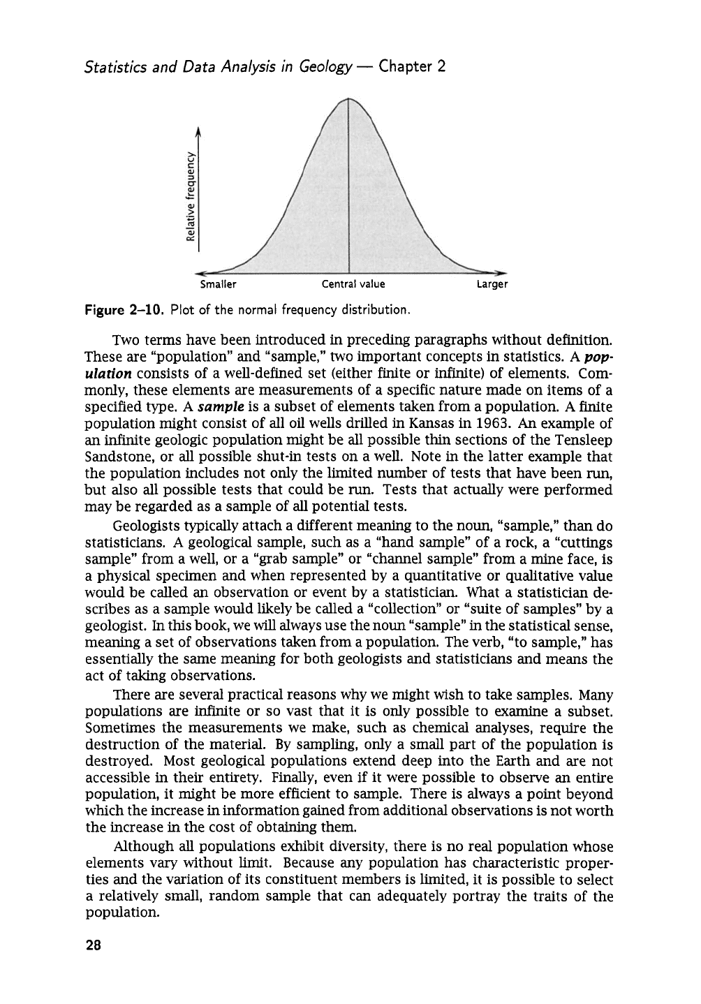
Smaller Central value Larger
Figure
2-10.
Plot
of
the normal frequency distribution.
Two terms have been introduced in preceding paragraphs without definition.
These are “population” and “sample,”
two
important concepts in statistics.
A
pop-
ulation
consists of a well-defined set (either finite
or
infinite) of elements. Com-
monly, these elements are measurements of a specific nature made on items of a
specified type.
A
sample
is a subset of elements taken from a population.
A
finite
population might consist of all
oil
wells drilled in Kansas in
1963.
An
example of
an
infinite geologic population might be all possible
thin
sections of the Tensleep
Sandstone,
or
all possible shut-in tests on a well. Note in the latter example that
the population includes not only the limited number of tests that have been
run,
but also all possible tests that could be
run.
Tests that actually were performed
may be regarded as a sample of all potential tests.
Geologists typically attach a different meaning to the noun, “sample,” than do
statisticians.
A
geological sample, such as a “hand sample”
of
a rock, a “cuttings
sample” from a well,
or
a “grab sample”
or
“channel sample” from a mine face, is
a physical specimen and when represented by a quantitative
or
qualitative value
would be called
an
observation
or
event by a statistician. What a statistician de-
scribes as a sample would likely be called a “collection”
or
“suite of samples” by a
geologist.
In
this book, we
will
always use the
noun
“sample”
in
the statistical sense,
meaning a set of observations taken from a population. The verb, “to sample,” has
essentially the same meaning for both geologists and statisticians and means the
act of taking observations.
There are several practical reasons why
we
might wish to take samples.
Many
populations are infinite
or
so
vast that it is only possible to examine a subset.
Sometimes the measurements we make, such as chemical analyses, require the
destruction of the material.
By
sampling, only a small part of the population is
destroyed. Most geological populations extend deep into the Earth and are not
accessible in their entirety. Finally, even if it were possible to observe
an
entire
population, it might be more efficient to sample. There is always a point beyond
which the increase in information gained from additional observations is not worth
the increase in the cost of obtaining them.
Although
all
populations exhibit diversity, there is no real population whose
elements vary without limit. Because
any
population has characteristic proper-
ties and the variation
of
its constituent members is limited, it is possible to select
a relatively small, random sample that can adequately portray the traits of the
population.
Elementary Statistics
If
observations with certain characteristics are systematically excluded from
the sample, deliberately or inadvertently, the sample
is
said to be
biased.
Suppose,
for example, we are interested in the porosity of a particular sandstone unit.
If
we exclude
all
loose and crumbly rocks from our sample because their porosity is
difficult to measure, we will alter the results of the study. It
is
likely that the range
of porosities
will
be truncated at the high end, biasing the sample toward low values
and giving
an
erroneously low estimate of the variation in porosity within the unit.
Samples should be drawn from populations in a random manner. This means
that each item
in
the population has
an
equal opportunity to be included
in
the
sample.
A
random sample
will
be unbiased, and as the sample size
is
increased,
will provide an increasingly refined picture
of
the nature of the population. Unfor-
tunately, obtaining a truly random sample may be impractical, as in the situation of
sampling a geologic unit that is partially buried. Samples within the unit at depth
do not have the same opportunity of being chosen as samples at outcrops. The
problems of sampling
in
such circumstances are complex; some of the references
at the end of this chapter discuss the effects of various sampling schemes and the
relative merits of different sampling designs. However, many geologic problems
involve the analysis of data collected without prior design. The interpretation of
subsurface structure from drill-hole data
is
a prominent example.
Statistics
Distributions have certain characteristics, such as their midpoint; measures indicat-
ing the amount of "spread"; and measures of symmetry of the distribution. These
characteristics
are
known
as
parameters
if they describe populations, and
statistics
if
they refer to samples. Statistics may be used to estimate parameters of parent
populations and to test hypotheses about populations.
Although summary statistics are important, sometimes we can learn more by
examining the distribution of the observations as shown on different plots and
graphs.
A
familiar form of display
is
the
histogram,
a bar chart in which a con-
tinuous variable
is
divided into discrete categories and the number or proportion
of observations that fall into each category is represented by the areas of the cor-
responding
bars.
(As
we have already seen, histograms are useful for showing
discrete distributions but now we are interested in their application to continuous
variables.) Usually the limits of categories are chosen
so
all of the histogram
in-
tervals
will
be the same width,
so
the heights of the bars also are proportional to
the numbers of observations within the categories represented by the bars.
If
the
vertical scale on the bar chart reads in number of observations, the graphic
is
called
a
frequency histogram.
If
the number of observations
in
each category are divided
by the total number of observations, the scale reads
in
percent and the bar chart is
a
relative frequency histogram.
Since a histogram covers the entire range of obser-
vations, the sum of the areas of
all
the bars
will
represent either the total number
of observations or
100%.
If
the observations have been selected in
an
unbiased,
representative manner, the sample histogram can be considered an approximation
of the underlying probability distribution.
The appearance of a histogram
is
strongly affected by our choice of the number
of categories and the starting value of the first category, especially
if
the sample
contains
only
a few observations. Dividing the data into a small number of cate-
gories increases the average number in each and the histogram
will
be relatively
29
Statistics and Data Analysis
in
Geology
-
Chapter
2
reproducible with repeated sampling. Unfortunately, such a histogram
will
contain
little detail and may not be particularly informative.
Increasing the number of
categories reveals more details of the distribution, but because each category will
contain fewer observations, the histogram
will
be less stable. The choice of origin
for histogram categories also may influence the shape of the histogram. Interactive
software allows the user to dynamically vary the width of the histogram intervals
and move the origin,
so
alternatives
can
be easily evaluated.
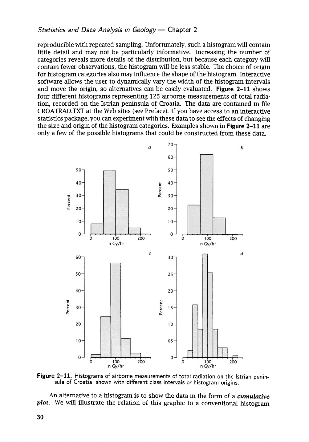
Figure
2-11
shows
four different histograms representing
125
airborne measurements of total radia-
tion, recorded on the Istrian peninsula of Croatia. The data are contained in file
CROATRAD.TXT at the Web sites (see Preface).
If
you have access to
an
interactive
statistics package, you can experiment with these data to see the effects of changing
the size and origin of the histogram categories. Examples shown
in
Figure
2-11
are
only a few of the possible histograms that could be constructed from these data.
Figure
2-11.
Histograms of airborne measurements of total radiation on the lstrian penin-
An
alternative to a histogram
is
to show the data in the form of a
cumulative
plot.
We
will
illustrate the relation of this graphic to a conventional histogram
sula
of
Croatia, shown with different class intervals or histogram origins.
30
Elementary Statistics
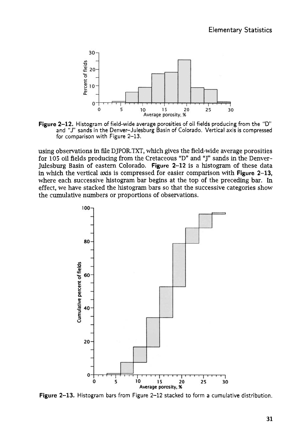
Figure
2-12.
Histogram of field-wide average porosities of oil fields producing from the
“D’
and
“J”
sands in the Denver-Julesburg Basin of Colorado. Vertical axis
is
compressed
for comparison with Figure
2-13.
using observations in file DJPOR.TXT, which gives the field-wide average porosities
for
105
oil
fields producing from the Cretaceous
“D”
and
“J”
sands
in
the Denver-
Julesburg Basin of eastern Colorado.
Figure
2-12
is
a histogram of these data
in
which the vertical
axis
is
compressed for easier comparison with
Figure
2-13,
where each successive histogram bar begins at the top of the preceding bar. In
effect, we have stacked the histogram bars
so
that the successive categories show
the cumulative numbers or proportions of observations.
Figure
2-13.
Histogram bars from Figure
2-12
stacked to form
a
cumulative distribution.
31
Statistics and Data Analysis in
Geology
-
Chapter
2
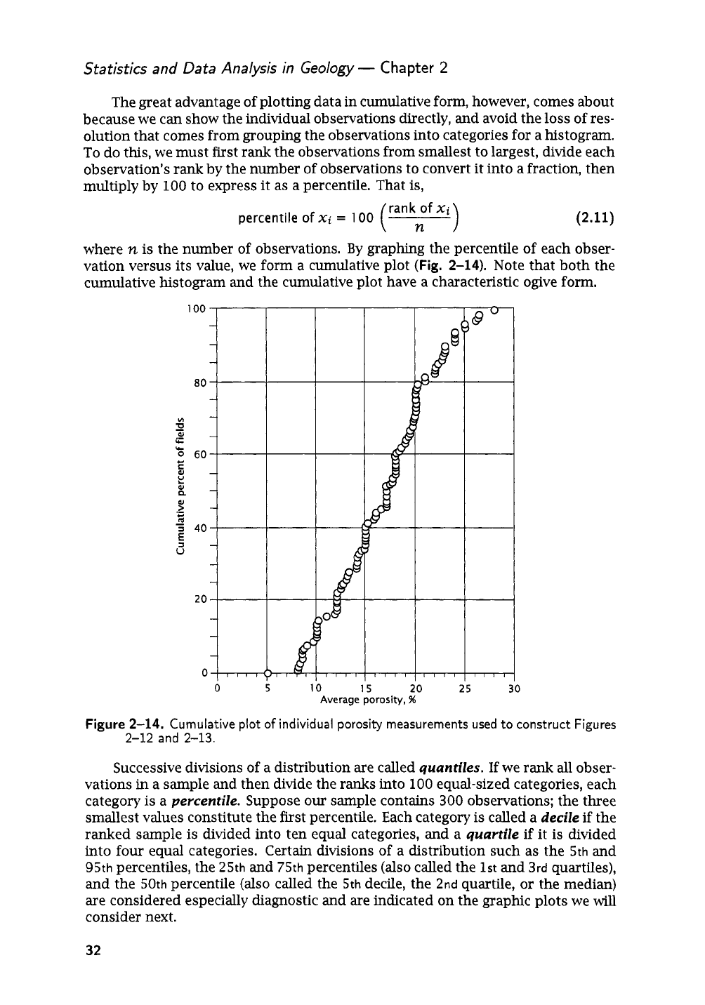
The great advantage of plotting data in cumulative form, however, comes about
because we
can
show the individual observations directly, and avoid the loss of res-
olution that comes from grouping the Observations into categories for a histogram.
To
do this, we must first rank the observations from smallest to largest, divide each
observation's rank by the number of observations to convert it into a fraction, then
multiply by
100
to express it as a percentile. That
is,
(
ran
","'
xi
)
percentile
of
Xi
=
100
(2.11)
where
n
is
the number of observations.
By
graphing the percentile
of
each obser-
vation versus its value, we form a cumulative plot
(Fig.
2-14).
Note that both the
cumulative histogram and the cumulative plot have a characteristic ogive form.
s
U
2ok
0
0
10
15
20
25
30
Average porosity,
%
Figure
2-14.
Cumulative plot
of
individual porosity measurements
used
to construct Figures
2-12
and
2-13.
Successive divisions of a distribution are called
quantizes.
If
we rank all obser-
vations
in
a sample and then divide the ranks into
100
equal-sized categories, each
category
is
a
percentile.
Suppose
our
sample contains
300
observations; the three
smallest values constitute the
first
percentile. Each category
is
called a
decile
if
the
ranked sample is divided into ten equal categories, and a
quartile
if it is divided
into four equal categories. Certain divisions of a distribution such as the
5th
and
95th
percentiles, the
25th
and
75th
percentiles (also called the
1st
and
3rd
quartiles),
and the
50th
percentile (also called the
5th
decile, the
2nd
quartile, or the median)
are considered especially diagnostic and are indicated on the graphic plots
we
will
consider next.
32
Elementary Statistics
Box-and-whiskev
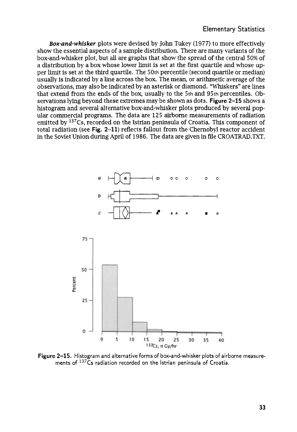
plots were devised by
John
Tukey
(1977)
to more effectively
show the essential aspects of a sample distribution. There are many variants of the
box-and-whisker plot, but all are graphs that show the spread of the central
50%
of
a distribution by a box whose lower limit is set at the first quartile and whose up-
per limit is set at the third quartile. The
50th
percentile (second quartile or median)
usually is indicated by a line across the box. The mean,
or
arithmetic average of the
observations, may also be indicated by an asterisk
or
diamond. “Whiskers”
are
lines
that extend from the ends of the box, usually to the
5th
and
95th
percentiles. Ob-
servations lying beyond these extremes may be shown as dots.
Figure
2-15
shows a
histogram and several alternative box-and-whisker plots produced by several pop-
ular commercial programs. The data are
125
airborne measurements of radiation
emitted by 13’Cs, recorded on the Istrian peninsula of Croatia. This component of
total radiation (see
Fig.
2-11)
reflects fallout from the Chernobyl reactor accident
in the Soviet Union during April of
1986.
The data
are
given in file
CROATRAD.TXT.
a
q&+m
00
0
00
bc
Figure
2-15.
Histogram and alternative forms
of
box-and-whisker plots
of
airborne measure-
ments
of
137Cs
radiation recorded on
the
lstrian peninsula of Croatia.
33
Statistics and Data Analysis
in
Geology
-
Chapter
2
Summary
Statistics
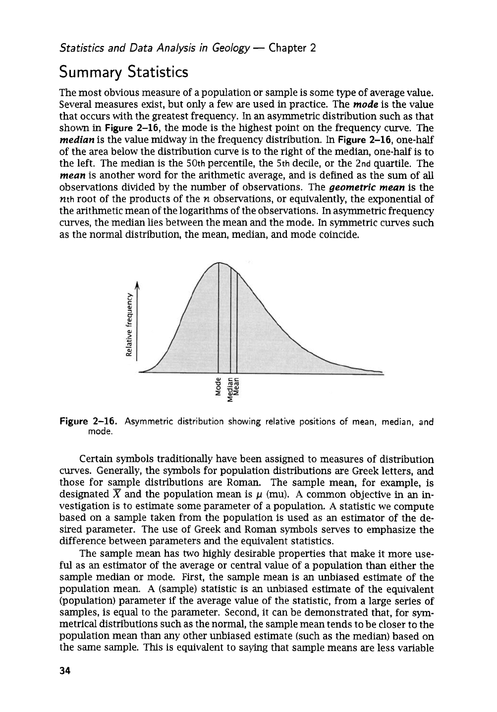
The most obvious measure of a population or sample is some type of average value.
Several measures exist, but only a few are used
in
practice. The
mode
is the value
that occurs with the greatest frequency. In an asymmetric distribution such as that
shown
in
Figure
2-16,
the mode is the highest point on the frequency curve. The
median
is the value midway
in
the frequency distribution.
In
Figure
2-16,
one-half
of the area below the distribution curve is to the right of the median, one-half is to
the left. The median is the
50th
percentile, the
5th
decile,
or
the
2nd
quartile. The
meun
is another word for the arithmetic average, and is defined as the
sum
of
all
observations divided by the number of observations. The
geometric meun
is the
nth
root of the products of the
n
observations,
or
equivalently, the exponential of
the arithmetic mean of the logarithms of the observations. In asymmetric frequency
curves, the median lies between the mean and the mode.
In
symmetric curves such
as the normal distribution, the mean, median, and mode coincide.
Figure
2-16.
Asymmetric distribution showing relative positions
of
mean, median, and
mode.
Certain symbols traditionally have been assigned to measures of distribution
curves. Generally, the symbols for population distributions are Greek letters, and
those for sample distributions
are
Roman. The sample mean, for example, is
designated
X
and the population mean is
p
(mu).
A
common objective
in
an
in-
vestigation is to estimate some parameter of a population.
A
statistic we compute
based on a sample taken from the population is used as an estimator of the de-
sired parameter. The use of Greek and Roman symbols serves to emphasize the
difference between parameters and the equivalent statistics.
The sample mean has
two
highly
desirable properties that make it more use-
ful as an estimator of the average
or
central value of a population than either the
sample median or mode. First, the sample mean is an unbiased estimate of the
population mean.
A
(sample) statistic is
an
unbiased estimate of the equivalent
(population) parameter
if
the average value of the statistic, from a large series of
samples, is equal to the parameter. Second, it can be demonstrated that, for sym-
metrical distributions such as the normal, the sample mean tends to be closer to the
population mean than any other unbiased estimate (such as the median) based on
the same sample. This is equivalent to saying that sample means
are
less variable
34
Elementary
Statistics
Table
2-1.
Chromium content
of
an Upper
Pennsylvanian shale
from
Kansas.
_-
Replicate
Cr
(ppm)
1 205
2
255
3
195
4
220
5
-
235
TOTAL=
1110
MEAN
=
1110/5=222
than sample medians, hence they
are
more efficient
in
estimating the population
parameter.
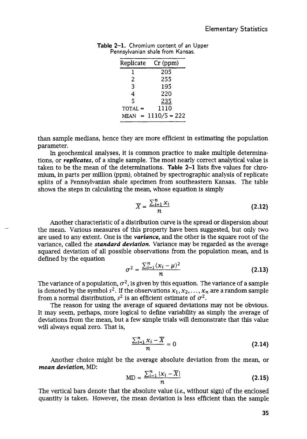
In geochemical analyses, it is common practice to make multiple determina-
tions,
or
replicates,
of a single sample. The most nearly correct analytical value is
taken to be the mean of the determinations.
Table
2-1
lists
five
values for chro-
mium,
in
parts per million (ppm), obtained by spectrographic analysis of replicate
splits of a Pennsylvanian shale specimen from southeastern Kansas. The table
shows the steps
in
calculating the mean, whose equation is simply
(2.12)
Another characteristic of a distribution curve is the spread
or
dispersion about
the mean. Various measures of this property have been suggested, but only two
are used to
any
extent. One is the
variance,
and the other is the square root of the
variance, called the
standard deviation.
Variance may be regarded as the average
squared deviation of all possible observations from the population mean, and is
defined bv the eauation
n
(2.13)
The variance of a population,
u2,
is given by this equation. The variance of
a
sample
is denoted by the symbol
s2.
If
the observations
XI,
XZ,
.
. .
,
xn
are a random sample
from a normal distribution,
s2
is an efficient estimate of
u2.
The reason for using the average of squared deviations may not be obvious.
It may seem, perhaps, more logical to define variability as simply the average of
deviations from the mean, but a few simple trials will demonstrate that this value
will always equal zero. That is,
(2.14)
Another choice might be the average absolute deviation from the
mean,
or
mean deviation,
MD:
-
cz,
1%
-XI
MD
=
n
(2.15)
The vertical bars denote that the absolute value
(i.e.,
without
sign)
of
the
enclosed
quantity is taken. However, the mean deviation is less efficient than the sample
35
Statistics and Data Analysis in Geology
-
Chapter
2
variance.
If
we take repeated samples, the mean deviations will be more variable
than variances calculated from the same samples. Although not intuitively obvious,
the variance has properties that make it far more useful than other measures of
scatter.
Because variance is the average squared deviation from the mean, its units are
the square of the units of the original measurements.
A
granite, for example, may
have feldspar phenocrysts whose longest axes have an average length of
13.2
mm
and a variance of
2.0 mm2.
Many
people may find themselves reluctant to regard
areas as
an
appropriate measurement
unit
for the dispersion of lengths! Fortu-
nately, in most instances where we are concerned with variance, it is standardized
or converted to a form independent of the measurement units.
This is a topic
discussed in greater detail elsewhere in this chapter.
To provide a statistic that describes dispersion or spread of data around the
mean, and is in the units of measurement of the data, we can calculate the
standard
deviation.
This is defined simply as the square root of variance and is symbolically
written as
CT
for the population parameter and
s
for the sample statistic. In equation
form,
(2.16)
A
small standard deviation indicates that observations are clustered tightly around
a central value. Conversely, a large standard deviation indicates that values
are
scattered widely about the mean and the tendency for central clustering is weak.
This is illustrated
in
Figure
2-17,
which shows two symmetric frequency curves
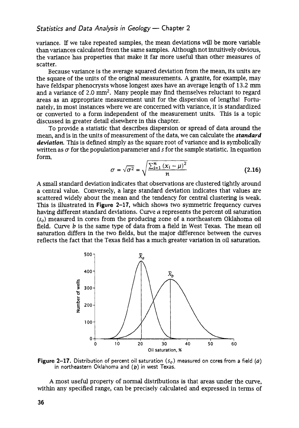
having different standard deviations. Curve
u
represents the percent
oil
saturation
(so)
measured in cores from the producing zone of a northeastern Oklahoma oil
field. Curve
b
is the same type of data from a field in West Texas. The mean
oil
saturation differs in the two fields, but the major difference between the curves
reflects the fact that the Texas field has a much greater variation
in
oil saturation.
500
1
P
Oil saturation,
%
Figure
2-17.
Distribution
of
percent oil saturation
(so)
measured on cores from a field
(a)
in northeastern Oklahoma and
(b)
in west Texas.
A
most useful property of normal distributions is that areas under the curve,
within
any
specified range, can be precisely calculated and expressed
in
terms of
36
Elementary Statistics
standard deviations from the mean.
For
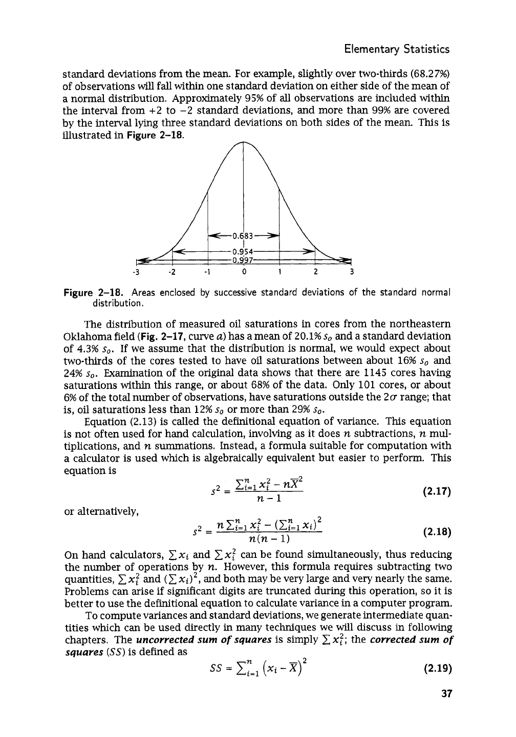
example, slightly over two-thirds
(68.27%)
of observations will fall
within
one standard deviation on either side of the mean of
a normal distribution. Approximately
95%
of
all observations are included within
the interval from
+2
to
-2
standard deviations, and more than
99%
are covered
by the interval lying three standard deviations on both sides of the mean. This is
illustrated in
Figure
2-18.
-0.683-
-3
-2
-1
0
1
2
3
Figure
2-18.
Areas enclosed by successive standard deviations
of
the standard normal
distribution.
The distribution of measured oil saturations in cores from the northeastern
Oklahoma field
(Fig.
2-17,
curve
u)
has
a
mean of
20.1%
so
and a standard deviation
of
4.3%
so.
If
we assume that the distribution is normal, we would expect about
two-thirds of the cores tested to have
oil
saturations between about
16%
so
and
24%
so.
Examination of the original data shows that there are
1145
cores having
saturations within this range, or about
68%
of the data. Only
101
cores,
or
about
6%
of
the total number of observations, have saturations outside the
2a
range; that
is,
oil
saturations less than
12%
so
or more than
29%
so.
Equation
(2.13)
is called the definitional equation of variance. This equation
is not often used for hand calculation, involving as it does
n
subtractions,
n
mul-
tiplications, and
n
summations. Instead, a formula suitable for computation with
a calculator is used which is algebraically equivalent but easier to perform. This
equation is
or
alternatively,
(2.17)
(2.18)
On hand calculators,
Cxi
and
Ex:
can be found simultaneously, thus reducing
the number
of
operations by
n.
However, this formula requires subtracting
two
quantities,
1
x;
and
(1
xi)2,
and both may be very large and very nearly the same.
Problems can arise
if
significant digits are truncated during this operation,
so
it
is
better to use the definitional equation to calculate variance in a computer program.
To compute variances and standard deviations, we generate intermediate quan-
tities which
can
be used directly in many techniques we will discuss in following
chapters. The
uncorrected sum
of
squares
is simply
2
x;;
the
corrected sum
of
squures
(SS)
is defined as
2
ss=
1:
t=l
(Xi-X)
(2.19)
37
Next Page
