Davis J.C. Statistics and Data Analysis in Geology (3rd ed.)
Подождите немного. Документ загружается.

Statistics and Data Analysis in Geology
-
Chapter
2
Number
of
holes
drilled
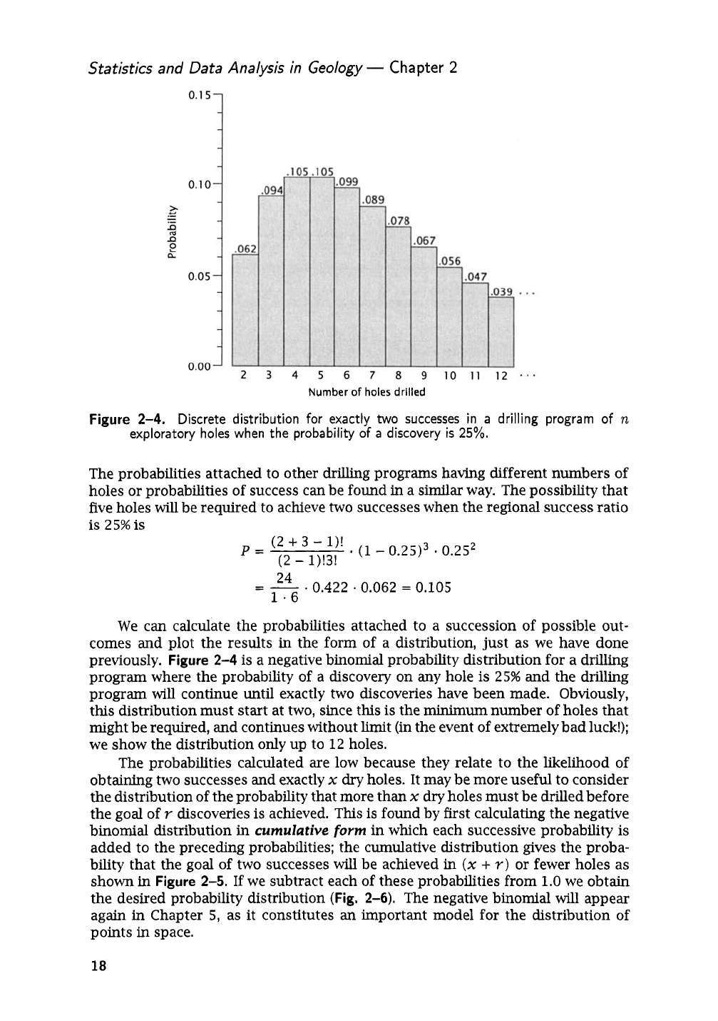
Figure
2-4.
Discrete distribution for exactly
two
successes in
a
drilling program of
n
exploratory holes when the probability
of
a
discovery
is
25%.
The probabilities attached to other drilling programs having different numbers of
holes or probabilities of success can be found
in
a similar way. The possibility that
five holes will be required to achieve two successes when the regional success ratio
is 25%
is
-
(1
-
0.25)3
*
0.2S2
(2
+
3
-
l)!
P=
(2
-
1)!3!
--.
-
24
0.422
-
0.062
=
0.105
1.6
We can calculate the probabilities attached to a succession of possible out-
comes and plot the results in the form of a distribution, just as we have done
previously.
Figure
2-4
is
a negative binomial probability distribution for a drilling
program where the probability of a discovery on
any
hole is
25%
and the drilling
program
will
continue until exactly two discoveries have been made. Obviously,
this distribution must start at two, since this
is
the
minimum
number of holes that
might be required, and continues without limit (in the event of extremely bad luck!);
we show the distribution only up to
12
holes.
The probabilities calculated are low because they relate to the likelihood of
obtaining two successes and exactly
x
dry
holes. It may be more useful to consider
the distribution of the probability that more than
x
dry holes must be drilled before
the goal of
Y
discoveries is achieved.
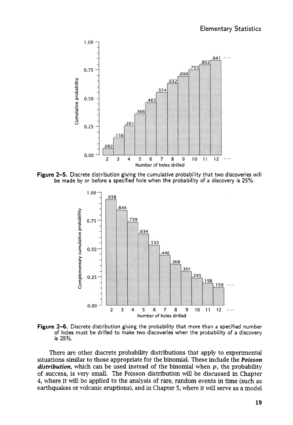
This
is
found by first calculating the negative
binomial distribution
in
cumulative
form
in
which each successive probability
is
added to the preceding probabilities; the cumulative distribution gives the proba-
bility that the goal of two successes will be achieved in
(x
+
Y)
or fewer holes as
shown in
Figure
2-5.
If
we subtract each of these probabilities from 1.0 we obtain
the desired probability distribution
(Fig.
2-6).
The negative binomial will appear
again in Chapter
5,
as it constitutes
an
important model for the distribution of
points
in
space.
18
Elementary
Statistics
Figure
2-5.
Discrete distribution giving the cumulative probability that
two
discoveries will
be made by or before
a
specified hole when
the
probability
of
a
discovery
is
25%.
Number
of
holes
drilled
Figure
2-6.
Discrete distribution giving
the
probability
that
more than
a
specified number
of holes must be drilled to make
two
discoveries when the probability of
a
discovery
is
25%.
There
are
other discrete probability distributions that apply to experimental
situations similar to those appropriate for the binomial. These include the
Poisson
distribution,
which can be used instead of the binomial when
p,
the probability
of
success, is very small. The Poisson distribution will be discussed in Chapter
4,
where it will be applied to the analysis
of
rare,
random events
in
time (such as
earthquakes or volcanic eruptions), and
in
Chapter
5,
where it
will
serve as a model
19
Statistics
and
Data Analysis in Geology
-
Chapter
2
for objects located randomly in space. The
geometric distribution
is
a special case
of the negative binomial, appropriate when interest is focused on the number of
trials prior to the initial success. The
multinomial distribution
is an extension of
the binomial where more than two mutually exclusive outcomes are possible. These
topics are extensively developed in most books on probability theory, such as those
by Parzen (1960) or Ash (1970).
An
important characteristic of
all
of the discrete probability distributions just
discussed is that the probability of success remains constant from trial to trial.
Statisticians discuss simple experiments called
sampling with replacement
in
which this assumption holds strictly true.
A
typical experiment would involve
an
urn filled with red and white balls; if a ball is selected at random, the probability it
will be red
is
equal to the proportion of red balls originally
in
the urn.
If
the ball is
then returned to the urn, the proportions of the two colors remain unchanged, and
the probability of drawing a red ball on a second trial remains unchanged as well.
The probability also will remain approximately constant if there are a very large
number of balls in the urn, even if those selected are not returned, because their
removal causes an infinitesimal change
in
the proportions among those remaining.
This latter condition usually is assumed to prevail in many geological situations
where discrete probability distributions are applied. In our binomial probability
example, the “urn” consists of the geologic basin where exploration is occurring,
and the red and white balls correspond to undiscovered reservoirs and barren areas.
As
long as the number of undrilled locations is large, and the number of prospects
that have been drilled (and hence “removed from the urn”)
is
small, the assump-
tion of constant probability of discovery seems reasonable. However, if a sampling
experiment is performed with a small number of colored balls initially in the urn
and those taken from the urn are not returned, the probabilities obviously change
with each draw. Such an experiment is called
sampling without replacement,
and
is governed by the discrete
hypergeometric distribution.
Geologic problems where
its use is appropriate are not common, but McCray (1975) presents
an
example
from geophysical exploration for petroleum.
In some circumstances it is possible to know the size of the population within
which discoveries
will
be made. Suppose
an
offshore concession contains ten well-
defined seismic features that seem to represent structures caused by movement
of
salt at depth. From experience in nearby offshore tracts, it is believed that about
40%
of such seismic features will prove to be productive structures. Because of
budgetary limitations, it is not possible to drill all of the features
in
the current
exploration program. The hypergeometric distribution can be used to estimate the
probabilities that specified numbers of discoveries
will
be made
if
only some
of
the
identified prospects are drilled.
The binomial distribution is not appropriate for this problem because the prob-
ability of a discovery changes with each exploratory hole.
If
there are four reser-
voirs distributed among the ten seismic features, the discovery of one reservoir
increases the odds against finding another because there are fewer remaining to
be discovered. Conversely, drilling a dry hole on a seismic feature increases the
probability that the remaining untested features
will
prove productive, because
one nonproductive feature has been eliminated from the population.
Calculating the hypergeometric probability consists simply of finding
all
of the
possible combinations of producing and dry features within the population,
and
then enumerating those combinations that yield the desired number
of
discoveries.
20
Elementary Statistics
The probability of making
x
discoveries
in
a drilling program of
n
holes, when
sampling from a population of
N
prospects of which
S
are believed to contain
reservoirs, is
This is the number of combinations of the reservoirs taken by the number of discov-
eries, times the number of combinations of barren anomalies taken by the number
of dry holes, all divided by the number of combinations of all the prospects taken
by the total number of holes in the drilling program.
The hypergeometric probability distribution can be applied to our offshore
concession that contains ten seismic features, of which four are likely to be struc-
tures containing reservoirs. Unfortunately, we cannot know in advance of drilling
which four of the ten features
will
prove productive.
If
the current season’s explo-
ration budget permits the drilling of only four of the prospects, we
can
determine
the probabilities attached to the various possible outcomes.
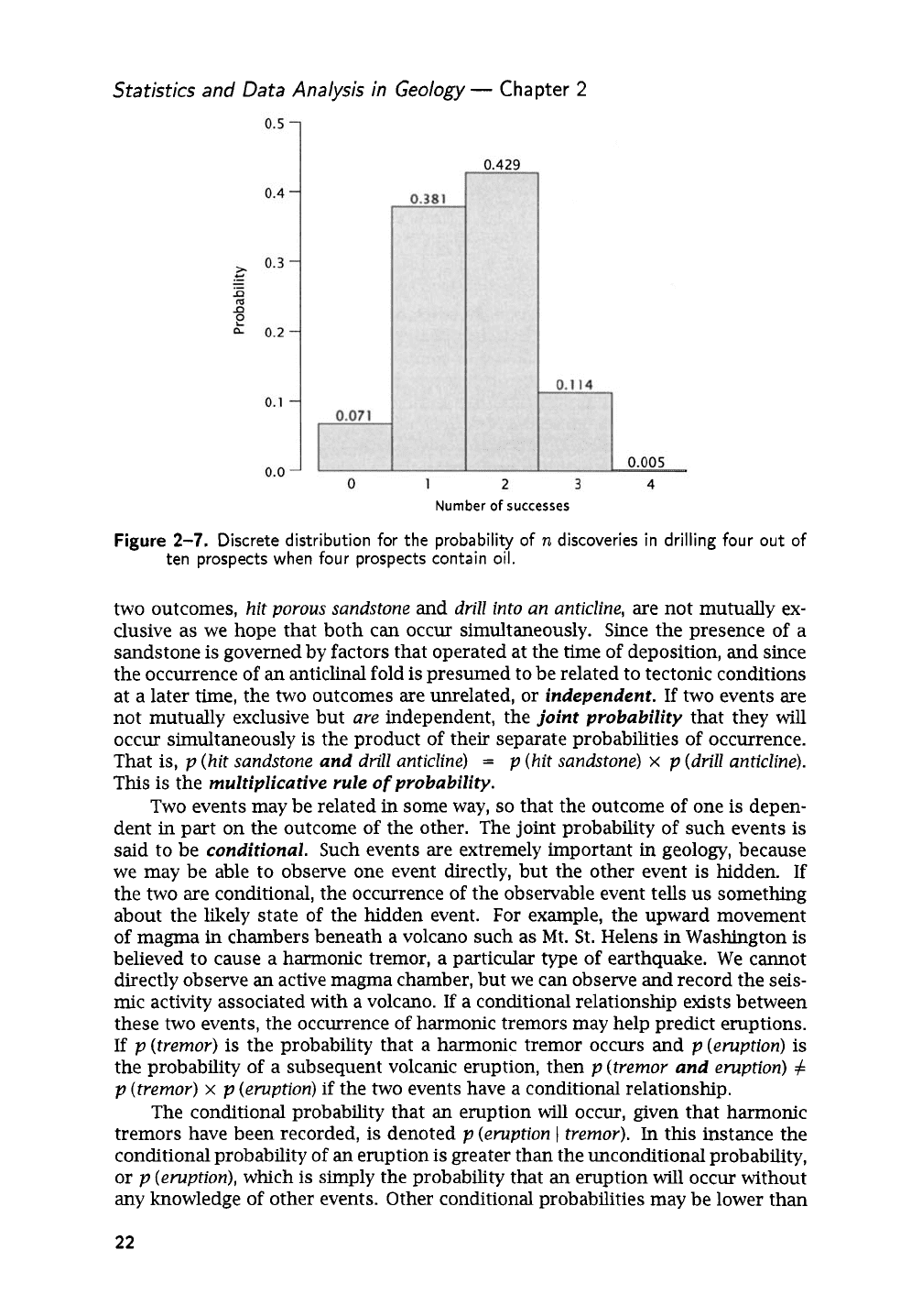
What is the probability that the drilling program
will
be a total failure, with
no
discoveries among the four features tested?
The probability of gambler’s ruin
is
approximately
7%.
What is the probability that
one discovery will be made?
The probability that one discovery will be made is
38%.
A
histogram can be prepared which shows the probabilities attached to all
possible outcomes
in
this exploration situation
(Fig.
2-7).
Note that the probability
of some success is
(1.00
-
0.07),
or
93%.
The preceding examples have addressed situations where there are only two
possible outcomes: a hole is
dry,
or
oil is discovered.
If
oil is found, the well cannot
be dry, and
vice versa.
Events in which the occurrence of one outcome precludes the
occurrence of the other outcome are
said
to be
mutually exclusive.
The probability
that one event
or
the other happens is the sum of their separate probabilities; that
is,
p
(discovery
or
dry
hole)
=
p
(discovery)
+
p
(dry hole).
This
is
called the
additive
rule
of
probability.
Events are not necessarily mutually exclusive.
For
example, we may be drilling
an
exploratory
hole
for
oil
or
gas in anticipation
of
hitting
a
porous
reservoir
sand-
stone
in
what we have interpreted as
an
anticlinal structure from seismic data. The
21
Statistics and Data Analysis in Geology
-
Chapter
2
Number
of
successes
Figure
2-7.
Discrete distribution for the probability of
n
discoveries in drilling four out of
ten prospects when four prospects contain oil.
two outcomes,
hit porous sandstone
and
dril2 into an anticline,
are not mutually ex-
clusive as we hope that both can occur simultaneously. Since the presence of a
sandstone
is
governed by factors that operated at the time of deposition,
and
since
the occurrence of
an
anticlinal fold is presumed to be related to tectonic conditions
at a later time, the two outcomes are unrelated, or
independent.
If
two events are
not mutually exclusive but
are
independent, the
joint probability
that they
will
occur simultaneously
is
the product of their separate probabilities
of
occurrence.
That
is,
p
(hit sandstone
and
drill anticline)
=
p
(hit sandstone)
x
p
(drill anticline).
This
is
the
muZtipZicative rule
of
probability.
Two events may be related in some way,
so
that the outcome of one
is
depen-
dent
in
part on the outcome of the other. The joint probability of such events
is
said to be
conditional.
Such events are extremely important in geology, because
we may be able to observe one event directly, but the other event is hidden.
If
the two are conditional, the occurrence of the observable event tells
us
something
about the likely state of the hidden event. For example, the upward movement
of
magma
in
chambers beneath a volcano such as Mt. St. Helens in Washington
is
believed to cause a harmonic tremor, a particular type
of
earthquake. We cannot
directly observe
an
active magma chamber, but we can observe and record the seis-
mic
activity associated with a volcano.
If
a conditional relationship exists between
these two events, the occurrence
of
harmonic tremors may help predict eruptions.
If
p(tremor)
is the probability that a harmonic tremor occurs and
p(eruption)
is
the probability of a subsequent volcanic eruption, then
p
(tremor
and
eruption)
#
p
(tremor)
x
p
(eruption)
if
the two events have a conditional relationship.
The conditional probability that
an
eruption
will
occur, given that harmonic
tremors have been recorded, is denoted
p
(eruption
1
tremor).
In
this instance the
conditional probability
of
an eruption is greater than the unconditional probability,
or
p
(eruption),
which
is
simply the probability that an eruption
will
occur without
any knowledge of other events. Other conditional probabilities may be lower than
22
Elementary Statistics
the corresponding unconditional probabilities (the probability of finding a fossil,
given that the terrain is igneous,
is
much lower than the unconditional probability
of finding a fossil). Obviously, geologists exploit conditional probabilities
in
all
phases of their work, whether this is done consciously
or
not.
The relationship between conditional and unconditionai probabilities can be
expressed by
Bayes’ theorem,
named for Thomas Bayes,
an
eighteenth century
En-
glish clergyman who investigated the manner
in
which probabilities change as more
information becomes available. Bayes’ basic equation is:
p(A,B)
=
p(BIA)p(A)
(2.7)
which states that
p(A,
B),
the
joint probability
that both events
A
and
B
occur, is
equal to the probability that
B
will occur given that
A
has already occurred, times
the probability that
A
will occur.
p(BIA)
is a conditional probability because it
expresses the probability that
B
will
occur conditional upon the circumstance that
A
has already occurred.
If
events
A
and
B
are related
(or
dependent), the fact that
A
has already transpired tells us something about the likelihood that
B
will then
occur. Conversely, it
is
also true that
Therefore, the two can be equated, giving
which may be rewritten as
This is a most useful relationship, because sometimes we know one form of con-
ditional probability but are interested in the other.
For
example, we may deter-
mine that mining districts often are characterized by the presence of abnormal
geomagnetic fields. However, we are more interested in the converse, which is the
probability that an area
will
prove to be mineralized, conditional upon the pres-
ence
of
a magnetic anomaly. We can gather estimates of the conditional probabil-
ity
p
(anomaly
I
mineralization)
and the unconditional probability
p
(mineralization)
from studies of
known
mining districts, but it may be more difficult to directly es-
timate
p
(mineralization
I
anomaly)
because this would require the examination of
geomagnetic anomalies that may not yet have been prospected:
If
there is an all-inclusive number of events
Bi
that are conditionally related to
event
A,
the probability that event
A
will
occur is simply the
sum
of the conditional
probabilities
p(AIBi)
times the probabilities that the events
Bi
occur. That is,
If
Equation
(2.9)
is substituted for
p(A)
in Bayes’ theorem, as given
in
Equation
(2.8),
we have the more general equation
(2.10)
23
Statistics and Data Analysis in Geology
-
Chapter
2
A
simple example involving two possible prior events,
B1
and
B2,
will illustrate
the use of Bayes’ theorem.
A
fragment of a hitherto
unknown
species of mosasaur
has been found in a stream bed
in
western Kansas, and a vertebrate paleontologist
would like to send a student field party out to search for more complete remains.
Unfortunately, the source of the fragment cannot be identified with certainty be-
cause the fossil was found below the junction of two dry stream tributaries. The
drainage basin of the larger stream contains about 18
mi2,
while the basin drained
by the smaller stream includes only about 10
mi2.
On the basis of just this
infor-
mation alone,
we
might postulate that the probability that the fragment came from
one of the drainage basins is proportional to the area of the basin,
or
10
p(B2)
=
-
=
0.36
28
However,
an
examination of a geologic report and map of the region discloses the
additional information that about
3
5%
of the outcropping Cretaceous rocks in the
larger basin
are
marine, while almost
80%
of the outcropping Cretaceous rocks
in
the smaller basin are marine. We may therefore postulate the conditional prob-
ability that, given a fossil is derived from basin
Bi,
it
will be a marine fossil, as
proportional to the percentage of the Cretaceous outcrop area
in
the basin that is
marine, or for basin
B1
and for basin
BZ
p(AIB1)
=
0.35
p(AIB2)
=
0.80
Using these probabilities and Bayes’ theorem, we can assess the conditional
probability that the fossil fragment came from basin
B1,
given that the fossil is
marine.
-
(0.35) (0.64)
-
(0.35) (0.64)
+
(0.80)
(0.36)
=
0.44
Similarly, the probability that the fossil came from the smaller basin
is
=
0.56
Fortunately for the students who must search the area, it seems somewhat
more likely that the fragment of marine fossil mosasaur
came
from the smaller
basin than from the larger. However, the differences
in
probability
are
very small
and, of course, depend upon the reasonableness of the assumptions used to esti-
mate the probabilities.
24
El
em
en
tary Statistics
Continuous
Random
Variables
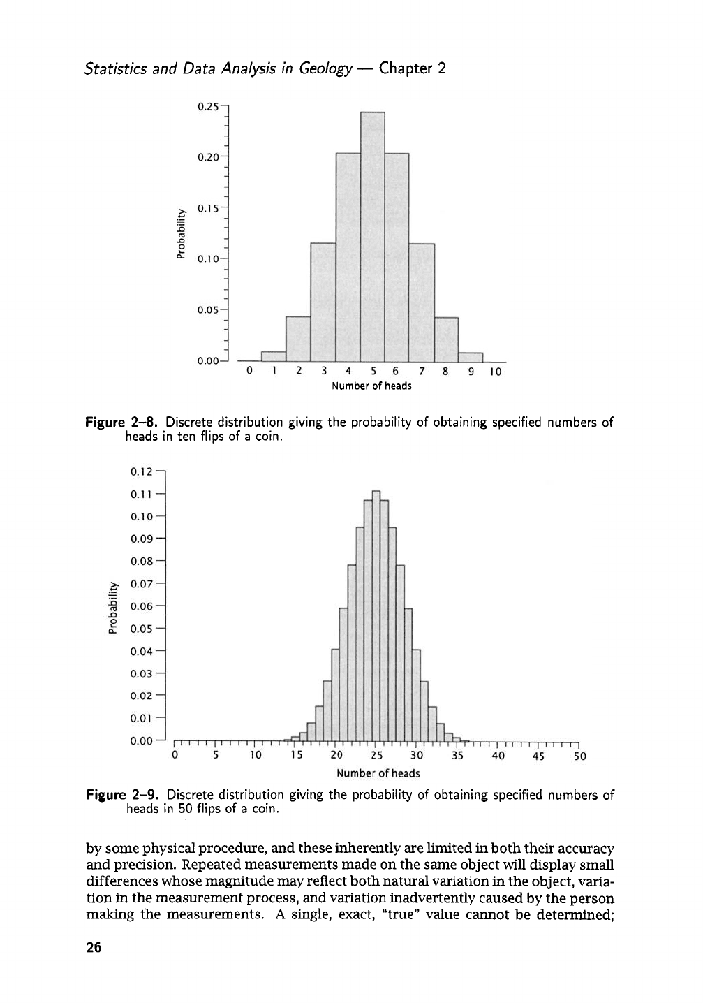
To introduce the next topic we must return briefly to the binomial distribution.
Figure
2-2
shows the probability distribution for
all
possible numbers of heads in
three flips of a coin.
A
similar experiment could be performed that would involve
a much larger number of trials.
Figure
2-8,
for example, gives the probabilities
associated with obtaining specified numbers of “successes” (or heads) in ten flips
of a coin, and
Figure
2-9
shows the probability distribution that describes out-
comes from
an
experiment involving
50
flips of a coin.
All
of the probabilities were
obtained either from binomial tables or calculated using the binomial equation.
In
each of these experiments, we have enumerated all possible numbers of
heads that we could obtain, from zero up to three, to ten, or to
50.
No
other com-
binations of heads and tails can occur. Therefore, the sum of
all
the probabilities
within each experiment must total 1.00, because we are absolutely certain to ob-
tain a result from among those enumerated. We can conveniently represent this by
setting the areas underneath histograms in
Figures
2-8
and
2-9
equal to
1.00,
as
was done
in
the histogram of
Figure
2-2.
The greater number of coin tosses
can
be accommodated only by making the histogram bars ever more narrow, and the
histogram becomes increasingly like a smooth and continuous curve. We can imag-
ine
an
ultimate experiment involving flips of
an
infinite number of coins, yielding
a histogram having
an
infinite number of bars of infinitesimal width. Then, the
histogram would be a continuous curve, and the horizontal
axis
would represent a
continuous, rather than discrete, variable.
In the coin-tossing experiment, we are dealing with discrete outcomes-that is,
specific combinations of heads and tails. In most experimental work, however, the
possible outcomes are not discrete. Rather, there is
an
infinite continuum of pos-
sible results that might be obtained. The range of possible outcomes may be finite
and in fact quite limited, but within the range the exact result that may appear
can-
not be predicted. Such events are called
continuous
random variables.
Suppose,
for example, we measure the length of the hinge line on a brachiopod and find it to
be 6
mm
long. However,
if
we perform our measurement using a binocular micro-
scope, we may obtain a length of 6.2
mm,
by using an optical comparator we may
measure 6.23
mm,
and with a scanning electron microscope, 6.231
mm.
A
contin-
uous variate can, in theory, be infinitely refined, which implies that we can always
find a difference between two measurements,
if
we conduct the measurements at
a fine enough scale. The corollary of this statement is that every outcome on a
continuous scale of measurement is unique, and that the probability of obtaining
a specific, exact result must be zero!
If
this is true, it would seem impossible to define probability on the basis of rel-
ative frequencies of occurrence. However, even though it is impossible to observe
a number of outcomes that are, for example, exactly 6.000..
.
000
mm,
it is entirely
feasible to obtain a set of measurements that
fall
within an interval around this
value. Even though the individual measurements are not precisely identical, they
are sufficiently close that we can regard them as belonging to the same class. In ef-
fect, we divide the continuous scale into discrete segments, and
can
then count the
number of events that occur within each interval. The narrower the class bound-
aries, the fewer the number of occurrences within the classes, and the lower the
estimates of the probabilities of occurrence.
When
dealing with discrete events, we
are
counting-a process that usually
can
be done with absolute precision. Continuous variables, however, must be measured
25
Statistics and Data Analysis in Geology
-
Chapter
2
Number
of
heads
Figure
2-8.
Discrete distribution giving the probability
of
obtaining specified numbers
of
heads in ten flips
of
a
coin.
Figure
2-9.
Discrete distribution giving the probability
of
obtaining specified numbers
of
heads in
50
flips
of
a
coin.
by some physical procedure, and these inherently are limited in both their accuracy
and precision. Repeated measurements made on the same object
will
display small
differences whose magnitude may reflect both natural variation
in
the object, varia-
tion in the measurement process, and variation inadvertently caused by the person
making the measurements.
A
single, exact, “true” value cannot be determined;
26
Elementary
Statistics
rather, we will observe a continuous distribution of possible values. This is a fun-
damental characteristic of a continuous random variable.
To further illustrate the nature of a continuous random variable,
we
can con-
sider the problem of performing permeability tests on core samples. Permeabilities
are determined by measuring the time required to force a certain amount of fluid,
under standardized conditions, through a piece of rock. Suppose one test indi-
cates a permeability of
108
md (millidarcies). Is this the “true” permeability of the
sample?
A
second test run on the same specimen may yield a permeability of
93
md, and
a
third test may register
112
md. The permeability that is recorded on
the instruments during
any
given
run
is affected by conditions which inevitably
vary
within
the instrument from test to test, vagaries of flow and turbulence that
occur within the sample, and inconsistencies in the performance of the test by the
operator.
No
single test
can
be taken as an exactly correct measure of the true
permeability. The various sources of fluctuation combine to yield a continuously
random variable, which we
are
sampling by making repeated measurements.
Variation induced into measurements by inaccuracy of instrumentation is most
apparent when repeated measurements
are
made on a single object or a test is
repeated without change. This variation is called
experimental emor.
In contrast,
variation may occur between members of a set if measurements
or
experiments
are
performed on a series
of
test objects. This is usually the variation that is of
scientific interest. Sometimes the two types of variations
are
hopelessly mixed
together,
or
confounded,
and the experimenter cannot determine what portion of
the variability is due to variation between his test objects and what is due to error.
Rather than a single piece of rock, suppose
we
have a sizable length
of
core
taken from a borehole through a sandstone body.
We
want to determine the per-
meability of the sandstone, but obviously cannot put 20
ft
of core into our per-
meability apparatus. Instead, we
cut
small plugs from the larger core at intervals
and determine the permeability of each. The variation
we
see is due
in
part to
dif-
ferences between the test plugs, but also results from differences in experimental
conditions. Devising methods to estimate the magnitude of different sources of
variation is one of the major tasks of statistics.
Repeated measurements on large samples drawn from natural populations may
produce a characteristic frequency distribution. Most values
are
clustered around
some central value, and the frequency of occurrence declines away from this central
point.
A
graph of the distribution
(Fig.
2-10)
appears bell-shaped, and is called
a
normal distribution.
It often is assumed that random variables are normally
distributed, and many statistical tests are based on this supposition.
As
with all frequency distributions, we may define the total area underneath
the normal curve as being equal to
1.00
(or if
we
wish, as
loo%),
so
we can calculate
the probability directly from the curve. You should note the similarity of the bell-
shaped continuous curve shown
in
Figure
2-10
to the histogram
of
the binomial
distribution in
Figure
2-9.
However, in
Figure
2-10
there is
an
infinite number of
subdivisions along the horizontal
axis
so
the probability of obtaining one exact,
specific event is essentially zero. Instead,
we
consider the probability of obtaining
a result within a specified range. This probability is proportional to the area
of
the frequency curve bounded by these limits.
If
our specified range is wide, we
are
more likely to observe
an
event within them;
if
the range
is
extremely
narrow,
observing an event is extremely unlikely.
27