Davis J.C. Statistics and Data Analysis in Geology (3rd ed.)
Подождите немного. Документ загружается.

Matrix Algebra
If
this seems unfamiliar, review the sections
in
an elementary algebra book that
deal with factoring and quadratic equations. Now, we can try the procedures just
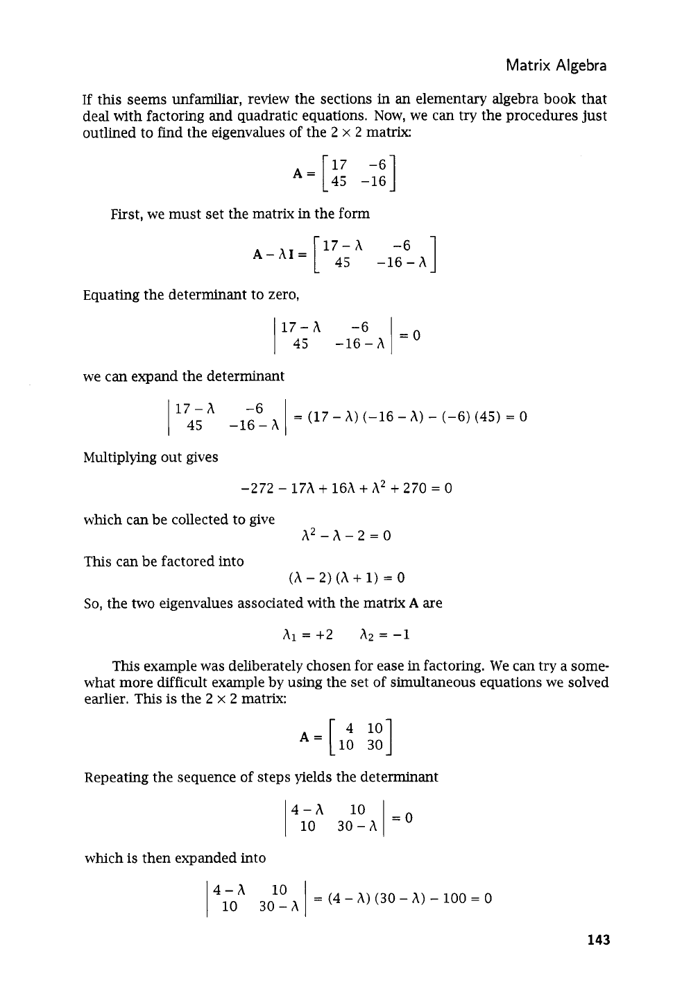
outlined to find the eigenvalues of the
2
x
2
matrix:
A=
[17
45
-16
-"]
First, we must set the matrix
in
the form
Equating the determinant to zero,
-6
l=o
1174
45
-16-h
we can expand the determinant
Multiplying out gives
-272
-
17h
+
16h
+
h2
+
270
=
0
which can be collected to give
This can be factored into
A2
-
h
-
2
=
0
(A
-
2)
(A
+
1)
=
0
So, the two eigenvalues associated with the matrix
A
are
This example was deliberately chosen for ease in factoring. We can try a some-
what more difficult example by using the set of simultaneous equations we solved
earlier. This
is
the
2
x
2
matrix:
A=
[
''1
10
30
Repeating the sequence of steps yields the determinant
which is then expanded into
I
4c;
3:!
1
=
(4
-A)
(30
-
A)
-
100
=
0
143

Statistics
and
Data Analysis in Geology-
Chapter
3
or
h2
-
34h
+
20
=
0
There are no obvious factors in the quadratic equation,
so
we must apply the
rule
for a general solution:
-
(-34)
c
J-342
-
4
x
1
x
20
34
+
JiDZ
2
-
=A=
-
-b+
J-
X=
2a
2x1
hi
=
33.4
A2
=
0.6
We
can
check
our
work
by
substituting the eigenvalues back into the determi-
nant to see
if
it is equal to zero,
within
the error introduced by round-off
So,
the eigenvalues we have found are correct
within
two decimal places.
Before
we
leave the computation of eigenvalues of
2
x
2
matrices, we should
consider one additional complication that may arise. Suppose we want the eigen-
values of the matrix
A=[
-6
2
41
3
Expressed as a determinant equal to zero, we have
which expands to
or
The
roots
of
this equation are
h2
-
5h
+
30
=
0
But this leads to equations involving the square roots of negative numbers:
=
2.5
+
4.9i
5+m
2
hl
=
=
2.5
-
4.9i
5-m
2
A2
=
144
Matrix
Algebra
20-h
-4
8
-40
8-h
-20
-60
12
-26-h
These are complex numbers, containing both real parts and imaginary parts which
include the imaginary number,
i
=
a.
Fortunately, a symmetric matrix always
yields real eigenvalues, and most of our computations involving eigenvalues and
eigenvectors
will
utilize covariance, correlation, or similarity matrices which are
always symmetrical.
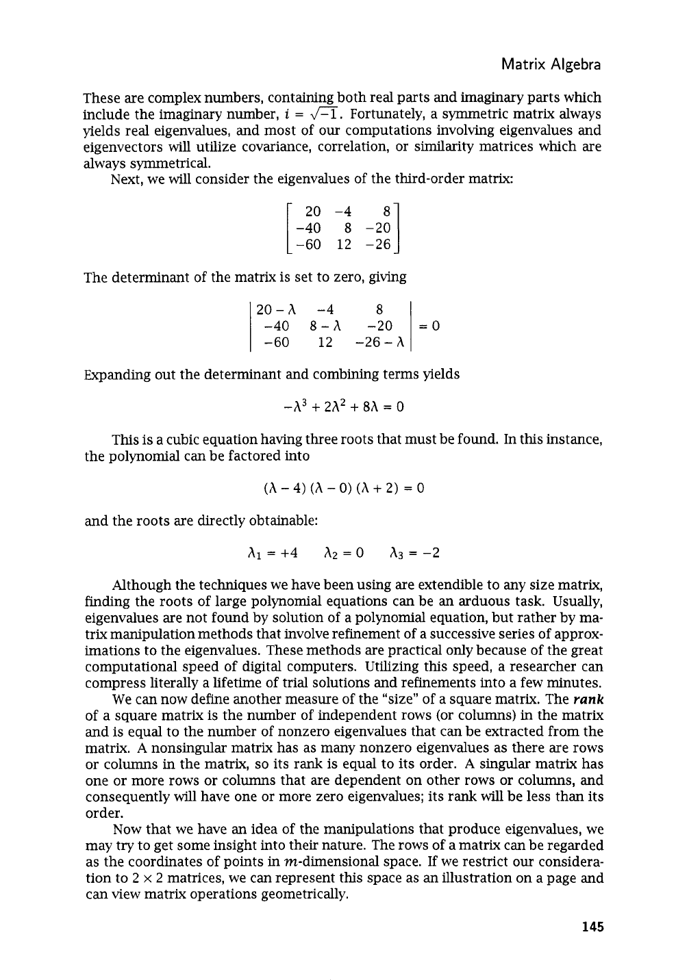
Next, we
will
consider the eigenvalues of the third-order matrix:
=O
20
-4
[
-40
8
-2:]
-60
12
-26
Expanding out the determinant and combining terms yields
-A3
+
2h2
+
8h
=
0
This
is
a cubic equation having three roots that must be found. In this instance,
the polynomial can be factored into
(A
-
4)
(A
-
0)
(A
+
2)
=
0
and the roots are directly obtainable:
h1=+4
h2=O
&=-2
Although the techniques we have been using are extendible to any size matrix,
finding the roots of large polynomial equations
can
be
an
arduous task. Usually,
eigenvalues are not found by solution of a polynomial equation, but rather by ma-
trix manipulation methods that involve refinement of a successive series of approx-
imations to the eigenvalues. These methods are practical only because of the great
computational speed of digital computers. Utilizing this speed, a researcher can
compress literally a lifetime of trial solutions and refinements into a few minutes.
We can now define another measure of the “size” of a square matrix. The
rank
of a square matrix
is
the number of independent rows (or columns) in the matrix
and
is
equal to the number of nonzero eigenvalues that can be extracted from the
matrix.
A
nonsingular matrix has as many nonzero eigenvalues as there are rows
or columns in the matrix,
so
its rank
is
equal to its order.
A
singular matrix has
one or more rows or columns that are dependent on other rows or columns, and
consequently will have one or more zero eigenvalues; its rank will be less than its
order.
Now that we have an idea of the manipulations that produce eigenvalues, we
may try to get some insight into their nature. The rows of
a
matrix can be regarded
as the coordinates of points in m-dimensional space.
If
we restrict
our
considera-
tion to
2
x
2
matrices, we can represent this space as an illustration on a page and
can view matrix operations geometrically.
145
Statistics and Data Analysis in Geology
-
Chapter
3
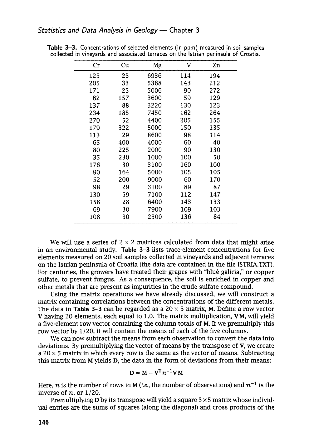
Table
3-3.
Concentrations
of
selected elements (in
ppm)
measured in
soil
samples
collected in vineyards and associated terraces on the lstrian peninsula
of
Croatia.
Cr cu Mg
V
Zn
125
25
205 33
171
25
62 157
137 88
2
34 185
2
70 52
179 322
113 29
65
400
80
225
35
230
176
30
90 164
52
200
98 29
130 59
158 28
69 30
108 30
6936
5368
5006
3600
3220
7450
4400
5000
8600
4000
2000
1000
3100
5000
9000
3 100
7100
6400
7900
2300
114 194
143
212
90
2
72
59 129
130 123
162
2
64
205
155
150 135
98 114
60
40
90 130
100
50
160 100
105 105
60
170
89 87
112
147
143 133
109 103
136 84
We
will
use a series of
2
x
2
matrices calculated from data that might
arise
in an environmental study.
Table
3-3
lists trace-element concentrations for five
elements measured on
20
soil
samples collected in vineyards and adjacent terraces
on the Istrian peninsula of Croatia (the data are contained in the file
1STRIA.TXT).
For centuries, the growers have treated their grapes with “blue galicia,” or copper
sulfate, to prevent fungus.
As
a consequence, the
soil
is enriched
in
copper and
other metals that are present as impurities in the crude sulfate compound.
Using the matrix operations we have already discussed, we will construct a
matrix containing correlations between the concentrations of the different metals.
The data in
Table
3-3
can be regarded as a
20
x
5
matrix,
M.
Define a row vector
V
having
20
elements, each equal to
1.0.
The matrix multiplication,
VM,
will yield
a five-element row vector containing the column totals of
M.
If
we premultiply this
row vector by
1
/20,
it
will contain the means of each of the five columns.
We can now subtract the means from each observation
to
convert the data into
deviations.
By
premultiplying the vector of means by the transpose
of
V,
we create
a
20
x
5
matrix
in
which every row is the same as the vector of means. Subtracting
this matrix from
M
yields
D,
the data
in
the form of deviations from their means:
D
=
M
-
VTn-lVM
Here,
n
is the number of rows in
M
(te.,
the number of observations) and
n-l
is the
inverse of
n,
or
1/20.
Premultiplying
D
by its transpose
will
yield a square
5
x
5
matrix whose individ-
ual entries are the
sums
of squares (along the diagonal) and cross products of the
146

Matrix Algebra
five elements, corrected for their means.
If
we divide a corrected
sum
of
squares
by
n
-
1
we obtain the variance, and if we divide a corrected
sum
of products by
n
-
1
we obtain the covariance. These are the elements of the covariance matrix,
S,
which we can compute by
s
=
(n
-
i1-l~~~
A
subset of
S
could serve our purposes (and the covariance matrix often
is
used in multivariate statistics), but the relationships will be clearer
if
we use the
correlation matrix,
R.
Correlations are simply covariances of standardized variables;
that is, observations from which the means have been removed and then divided
by the standard deviation.
In
matrix
D,
the means have already been removed. We
can,
in
effect, divide by the appropriate standard deviations if we create a
5
x
5
matrix,
C,
whose diagonal elements are the square roots of the variances found on
the diagonal
of
S,
and whose off-diagonal elements are all
0.0.
If
we invert
C
and
premultiply by
D,
each element of
D
will
be divided by the standard deviation of its
column. Call the result
U,
a
20
x
5
matrix of standardized values;
U
=
DC-’
We can calculate the correlation matrix by repeating the procedure we used to
find
S,
substituting
U
for
D:
R
=
(n
-
l)-lUTU
1
1
0.595
-0.28
0.456
0.242
1
1
-0.312
0.141
0.85
0.595
-0.312
1
-0.201
-0.33 -0.28
R
=
0.141
-0.201
1
-0.029 0.456
0.85 -0.33 -0.029
1
0.242
To graphically illustrate matrix relationships, we must confine ourselves to
2
x
2
matrices, which we
can
extract from
R.
Copper and zinc are recorded in the
second and fifth columns of
M,
and
so
their correlations are the elements
Yi,j
whose
subscripts are
2
and
5:
1
Rcu,,.,,
=
[
Y212
“g5]
=
[
1
-0.28
r5,2
r5,S
-0.28
1
If
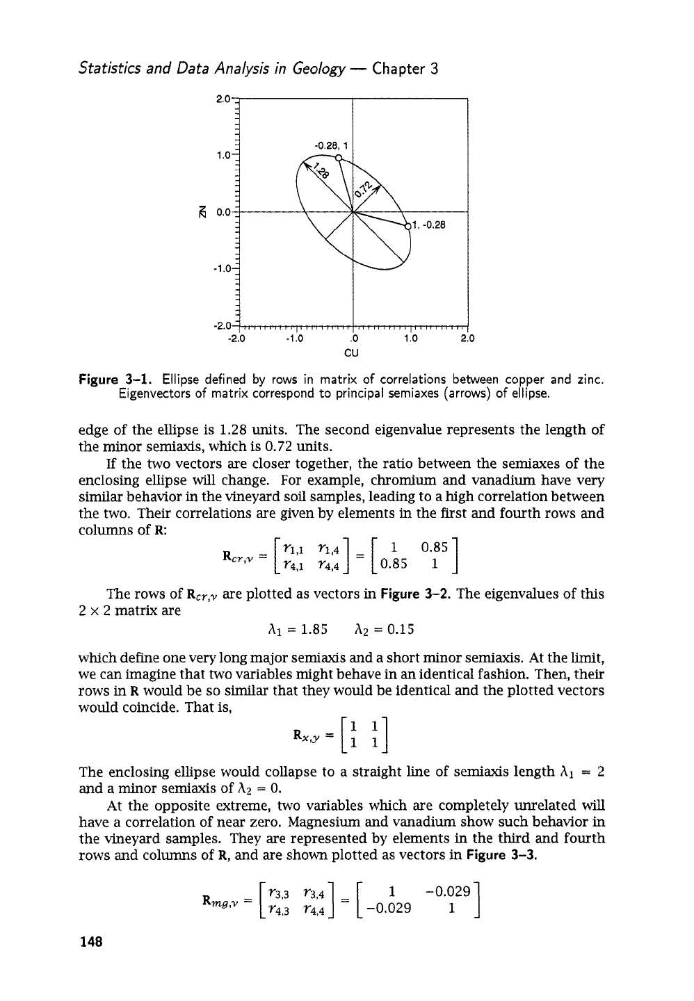
we regard the rows as vectors in
X
and
Y,
we can plot each row as the tip
of a vector that extends from the origin.
In
Figure
3-1,
the tip of each vector
is indicated by an open circle, labeled with its coordmates. The ends of the two
vectors lie on an ellipse whose center is at the origin
of
the coordinate system and
which just encloses the tips of the vectors. The eigenvalues of the
2
x
2
matrix
R,,,,,
represent the magnitudes, or lengths, of the major and minor semiaxes of
the ellipse.
In
this example, the eigenvalues are
hi
=
1.28
A2
=
0.72
Gould refers to the relative lengths
of
the semiaxes as a measure of the “stretch-
ability” of the enclosing ellipse. The semiaxes are shown by arrows on
Figure
3-1.
The first eigenvalue represents the major semiaxis whose length from center to
147
Statistics and Data Analysis in
Geology
-
Chapter
3
1
.o:
-
-0.28,
1
I
1
.o:
-
3
-0.28,
1
Figure
3-1.
Ellipse defined
by
rows in matrix
of
correlations between copper and zinc.
Eigenvectors
of
matrix correspond
to
principal semiaxes (arrows)
of
ellipse.
-2.0-,,
edge of the ellipse is
1.28
units. The second eigenvalue represents the length of
the minor semiaxis, which is
0.72
units.
If
the
two
vectors are closer together, the ratio between the semiaxes of the
enclosing ellipse will change. For example, chromium and vanadium have very
similar
behavior
in
the vineyard
soil
samples, leading to a high correlation between
the two. Their correlations are given by elements in the first and fourth rows and
I,,,,,,
II
,,,,,,,,I,,
4
IIIIIIIII
I,,,,
I
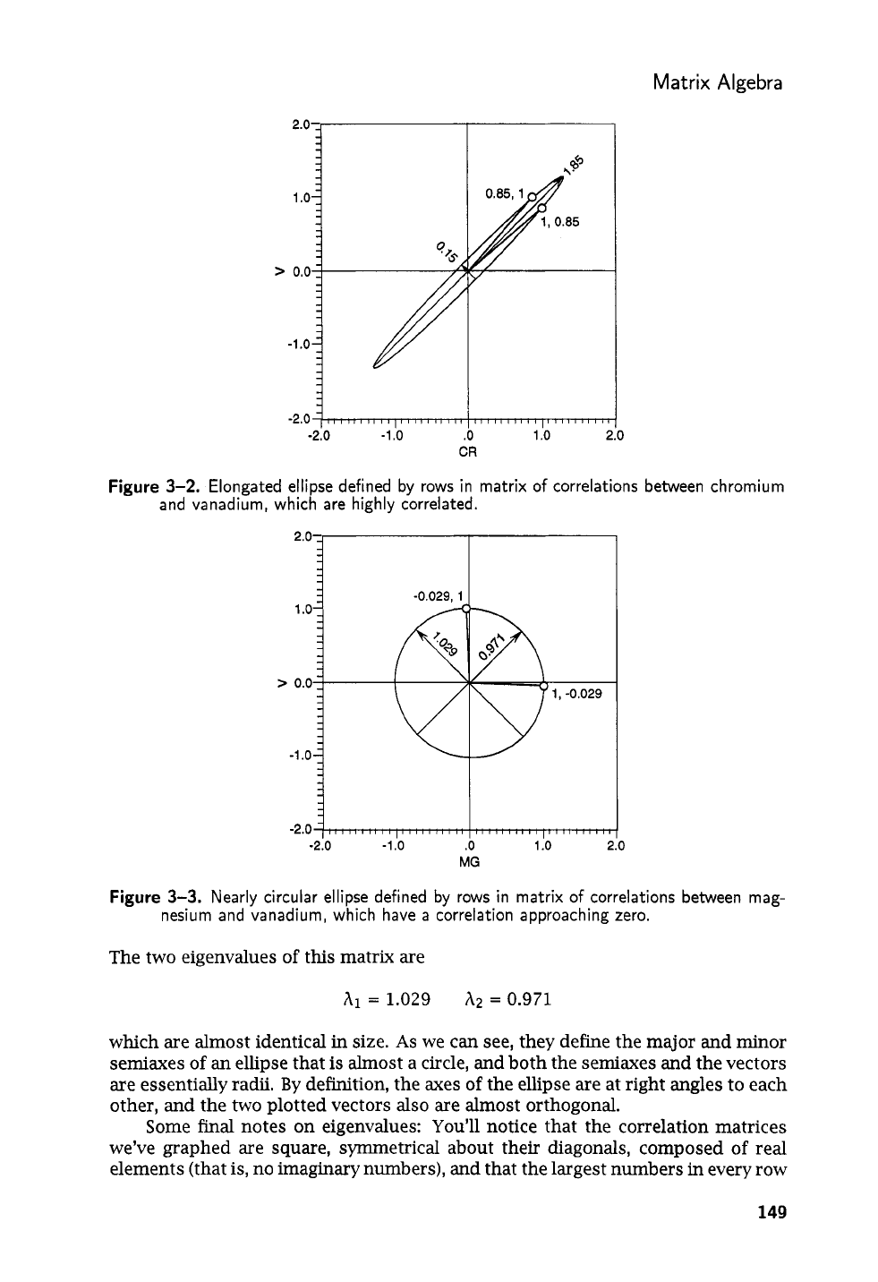
The rows of
RCY,,,
are plotted as vectors
in
Figure
3-2.
The eigenvalues of this
2
x
2
matrix are
hi
=
1.85
hz
=
0.15
-2.0-,,
which define one very long major semiaxis and a short minor semiaxis. At the limit,
we
can
imagine that two variables might behave in
an
identical fashion. Then, their
rows
in
R
would be
so
similar that they would be identical and the plotted vectors
would coincide. That is,
I,,,,,,
II
,,,,,,,,,I
4
IIIIIIIII
I,,,,
I
The enclosing ellipse would collapse to a straight line of semiaxis length
hl
=
2
and a minor semiaxis of
hz
=
0.
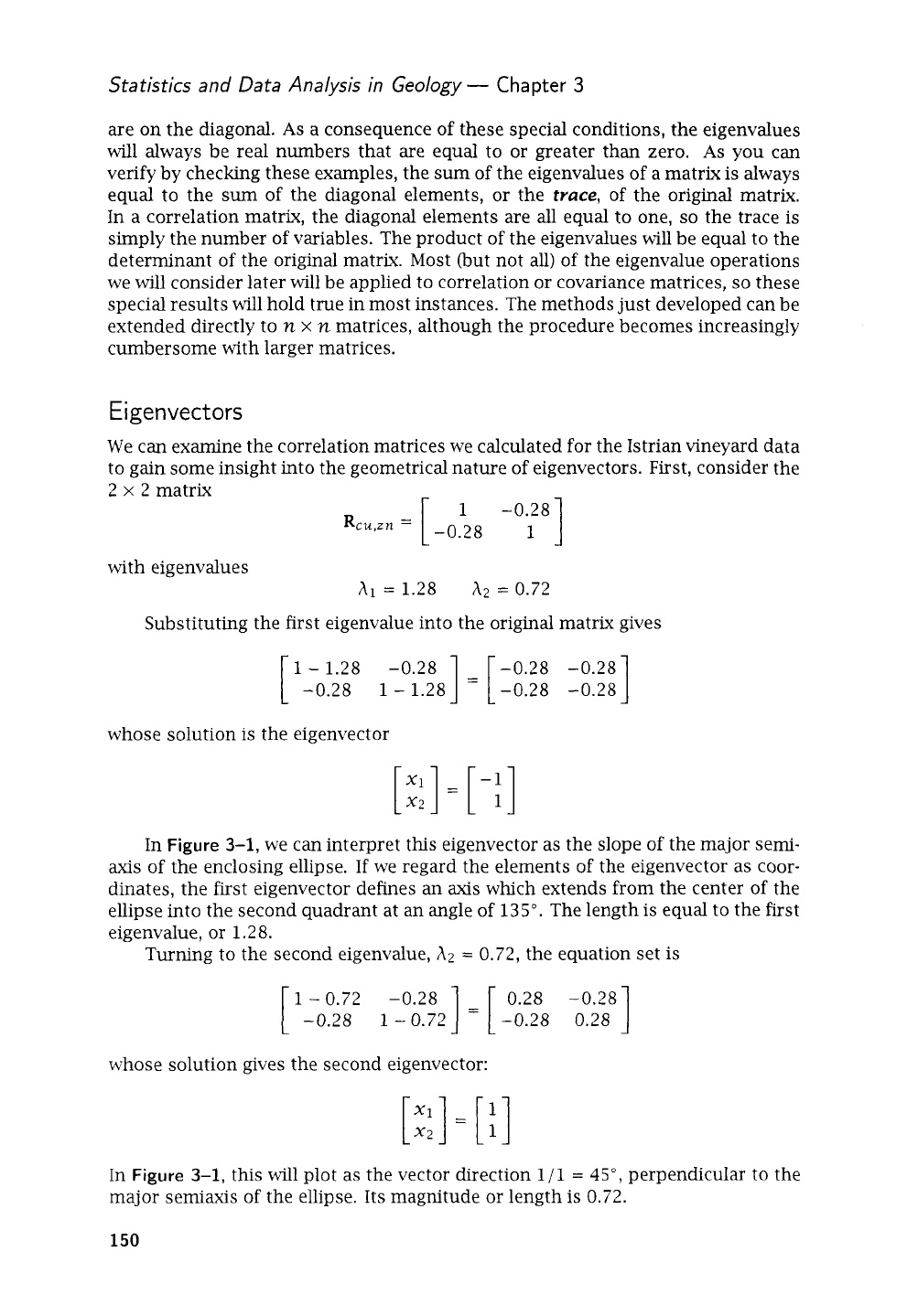
At the opposite extreme, two variables which are completely unrelated
will
have a correlation of near zero. Magnesium and vanadium show such behavior in
the vineyard samples. They are represented by elements in the third and fourth
rows and columns
of
R,
and are shown plotted as vectors in
Figure
3-3.
148
Matrix Algebra
3
Figure
3-2.
Elongated ellipse defined by rows in matrix
of
correlations between chromium
and vanadium, which are highly correlated.
2’o-:
-2.0
-2.0
-1
.o
.O
1
.o
2
MG
0
Figure
3-3.
Nearly circular ellipse defined by rows in matrix
of
correlations between mag-
nesium and vanadium, which have
a
correlation approaching zero.
The two eigenvalues
of
this matrix are
hi
=
1.029
A2
=
0.971
which are almost identical
in
size.
As
we can
see,
they define the major and minor
semiaxes
of
an
ellipse that is almost a circle, and both the semiaxes and the vectors
are essentially radii. By definition, the axes
of
the ellipse are at right angles to each
other, and the two plotted vectors also are almost orthogonal.
Some final notes on eigenvalues: You’ll notice that the correlation matrices
we’ve graphed are square, symmetrical about their diagonals, composed
of
real
elements (that
is,
no imaginary numbers), and that the largest numbers
in
every row
149
Statistics and Data Analysis in Geology
-
Chapter
3
are on the diagonal.
As
a consequence
of
these special conditions, the eigenvalues
will always be real numbers that are equal to or greater than zero.
As
you can
verify by checlung these examples, the sum of the eigenvalues of a matrix is always
equal to the
sum
of the diagonal elements, or the
trace,
of
the original matrix.
In a correlation matrix, the diagonal elements are all equal
to
one,
so
the trace
is
simply the number
of
variables. The product of the eigenvalues
will
be equal to the
determinant of the original matrix. Most (but not all) of the eigenvalue operations
we
will
consider later will be applied to correlation or covariance matrices,
so
these
special results will hold true in most instances. The methods just developed can be
extended directly to
n
x
n
matrices, although the procedure becomes increasingly
cumbersome with larger matrices.
E
igenvect
ors
We can examine the correlation matrices we calculated for the Istrian vineyard data
to gain some insight into the geometrical nature of eigenvectors. First, consider the
2
x
2
matrix
with eigenvalues
A1
=
1.28
A2
=
0.72
Substituting the first eigenvalue into the original matrix gives
1
1
-
1.28
-0.28
]
=
[
-0.28 -0.28
-0.28
1
-
1.28 -0.28 -0.28
whose solution is the eigenvector
[
4
=
[
-:]
In
Figure
3-1,
we can interpret this eigenvector as the slope
of
the major semi-
axis
of the enclosing ellipse.
If
we regard the elements of the eigenvector as coor-
dinates, the first eigenvector defines
an
axis
whch extends from the center of the
ellipse into the second quadrant at an angle of
135".
The length is equal to the first
eigenvalue, or
1.28.
Turning to the second eigenvalue, A2
=
0.72,
the equation set is
1
1
-
0.72
-0.28
]
=
[
0.28
-0.28
-0.28
1
-
0.72 -0.28 0.28
whose solution gives the second eigenvector:
[::I
=
[
:]
In
Figure
3-1,
ths will plot as the vector drection
l/l
=
45",
perpendicular to the
major semiaxis of the ellipse. Its magnitude or length is
0.72.
150
Matrix
Algebra
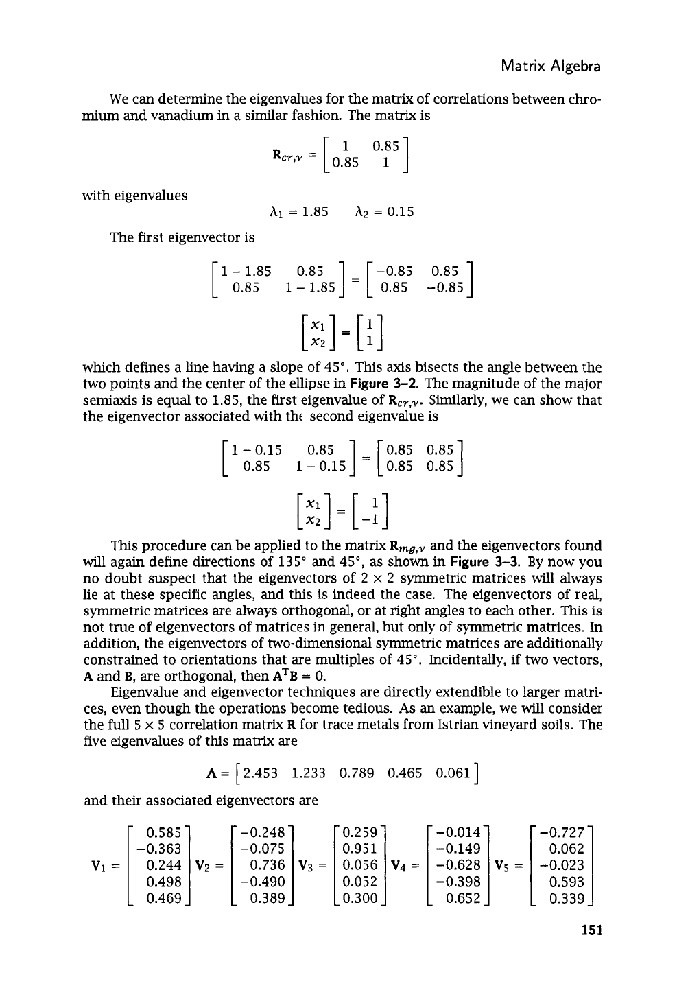
We can determine the eigenvalues for the matrix of correlations between chro-
mi=
and vanadium
in
a similar fashion. The matrix
is
with eigenvalues
hi
=
1.85
A2
=
0.15
The first eigenvector
is
1
-
1.85 0.85
1
=
1-0.85 0.85
1
1
0.85
1
-
1.85 0.85 -0.85
L
AL
A
[::I
=
[:I
which defines a line having a slope of
45".
This
axis
bisects the angle between the
two points and the center of the ellipse
in
Figure
3-2.
The magnitude of the major
semiaxis
is
equal to
1.85,
the first eigenvalue of
RC7,,,.
Similarly, we can show that
the eigenvector associated with th( second eigenvalue
is
1-0.15
0.85
]
=
[
0.85 0.851
0.85
1
-
0.15 0.85 0.85
[
::I
=
[-:I
This
procedure
can
be applied to the matrix
Rmg,,,
and the eigenvectors found
will again define directions
of
135"
and
45",
as shown in Figure 3-3. By now you
no doubt suspect that the eigenvectors
of
2
x
2
symmetric matrices
will
always
lie at these specific angles, and this
is
indeed the case. The eigenvectors of real,
symmetric matrices are always orthogonal, or at right angles to each other. This
is
not true
of
eigenvectors of matrices
in
general, but only of symmetric matrices. In
addition, the eigenvectors of two-dimensional symmetric matrices are additionally
constrained to orientations that are multiples of
45".
Incidentally,
if
two
vectors,
A
and
B,
are orthogonal, then
ATB
=
0.
Eigenvalue and eigenvector techniques are directly extendible to larger matri-
ces, even though the operations become tedious.
As
an example, we will consider
the full
5
x
5
correlation matrix
R
for trace metals from Istrian vineyard soils. The
five eigenvalues of this matrix are
A=
12.453 1.233 0.789 0.465
L
and their associated eigenvectors are
0.585
-0.363
0.498
0.469
-0.248
-0.075
Vp
=
[
0.736
0.389
-0.490
0.259
0.95
1
0.052
0.300
v4
=
0.061
]
1::!::]
[
-0.727 0.062
-0.628
Vs
=
-0.023
-0.398 0.593
0.652 0.339
151
Statistics and Data Analysis in Geology
-
Chapter
3
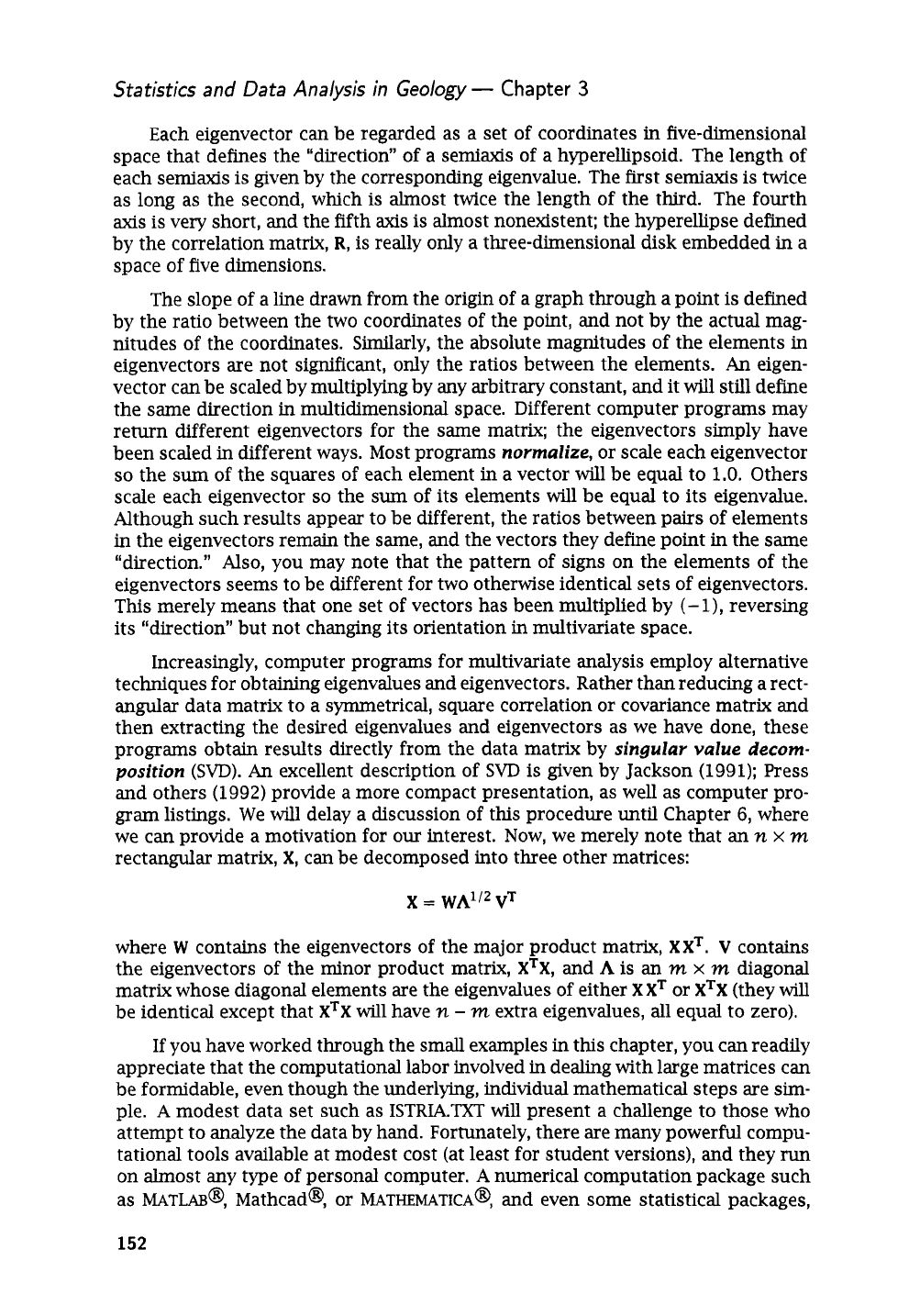
Each eigenvector
can
be regarded as a set of coordinates
in
five-dimensional
space that defines the “direction” of a semiaxis of a hyperellipsoid. The length of
each semiaxis is given by the corresponding eigenvalue. The first semiaxis is twice
as long as the second, which is almost twice the length of the third. The fourth
axis
is very short, and the fifth
axis
is almost nonexistent; the hyperellipse defined
by the correlation matrix,
R,
is really only a three-dimensional disk embedded in a
space of five dimensions.
The slope of a line drawn from the origin of a graph through a point is defined
by the ratio between the two coordinates of the point, and not by the actual mag-
nitudes of the coordinates. Similarly, the absolute magnitudes of the elements
in
eigenvectors are not significant, only the ratios between the elements.
An
eigen-
vector
can
be scaled by multiplying by
any
arbitrary constant, and it will still define
the same direction in multidimensional space. Different computer programs may
return different eigenvectors for the same matrix; the eigenvectors simply have
been scaled in different ways. Most programs
normalize,
or scale each eigenvector
so
the sum of the squares of each element in a vector will be equal to
1.0.
Others
scale each eigenvector
so
the sum of its elements will be equal
to
its eigenvalue.
Although such results appear to be different, the ratios between pairs of elements
in
the eigenvectors remain the same, and the vectors they define point in the same
“direction.”
Also,
you may note that the pattern of signs on the elements of the
eigenvectors seems to be different for two otherwise identical sets of eigenvectors.
This merely means that one set of vectors has been multiplied by
(-l),
reversing
its “direction” but not changing its orientation in multivariate space.
Increasingly, computer programs for multivariate analysis employ alternative
techniques for obtaining eigenvalues and eigenvectors. Rather than reducing a rect-
angular data matrix to a symmetrical, square correlation or covariance matrix and
then extracting the desired eigenvalues and eigenvectors as we have done, these
programs obtain results directly from the data matrix by
singular value
decom-
position
(SVD).
An
excellent description of
SVD
is given by Jackson (1991); Press
and others (1992) provide a more compact presentation, as well as computer pro-
gram listings.
We
will delay a discussion
of
this procedure until Chapter
6,
where
we
can
provide a motivation for
our
interest. Now, we merely note that an
n
x
m
rectangular matrix,
X,
can be decomposed into three other matrices:
where
W
contains the eigenvectors
of
the major product matrix,
XXT.
V
contains
the eigenvectors of the minor product matrix,
XTX,
and
A
is an
m
x
m
diagonal
matrix whose diagonal elements are the eigenvalues
of
either
XXT
or
XTX
(they will
be identical except that
XTX
will have
n
-
m
extra eigenvalues, all equal to zero).
If
you have worked through the small examples
in
this chapter, you can readily
appreciate that the computational labor involved in dealing with large matrices can
be formidable, even though the underlying, individual mathematical steps are sim-
ple.
A
modest data set such as
1STRIA.m
will present a challenge to those who
attempt to analyze the data by hand. Fortunately, there are many powerful compu-
tational tools available at modest cost (at least for student versions), and they
run
on almost
any
type of personal computer.
A
numerical computation package such
as
MATLAB@,
Mathcad@,
or
MATHEMATICA@,
and even some statistical packages,
152
