Davis J.C. Statistics and Data Analysis in Geology (3rd ed.)
Подождите немного. Документ загружается.

Statistics and Data Analysis in Geology
-
Chapter
6
against
The null hypothesis states that the mean vector of the parent population of the
first sample is the same as the mean vector of the parent population from which
the second sample was drawn.
The test we must use is a multivariate equivalent of Equation
(2.48)
on p.
73.
In that two-sample t-test, we used a pooled estimate of the population variance
based on both samples. Accordingly, we must compute a pooled estimate,
S,,
of
the common variance-covariance matrix from
our
two multivariate samples.
This
is
done by calculating a matrix of sums of squares and products for each sample.
We can use the terminology of discriminant functions and denote the matrix of
sums
of
squares and cross products of sample
A
as
SA;
similarly, the matrix from
sample
B
is
SB.
The pooled estimate of the variance-covariance matrix is
H1
:
P1
#Po
S,
=
(nA
+
nB
-
2)-l
(sA
+
sB)
(6.32)
We must next find the difference between the two mean vectors,
D
=
EA
-
XB.
Our
T2
test has the form
nAnB
D‘S,
lD
T2
=
nA
+
nB
(6.33)
The significance of the
T2
test statistic can be determined by the F-transformation:
T2
nA
+
nB
-
m
-
1
(nA
+
nB
-
2)m
F=
(6.34)
which has
m
and
(nA
+
nB
-
m
-
1)
degrees of freedom (Morrison, 1990).
Eq
ua
I
ity
of
varia nce-covaria nce matrices
An
underlying assumption in the two preceding tests
is
that the samples are drawn
from populations having the same variance-covariance matrix. This is the multi-
variate equivalent of the assumption of equal populationvariances necessary to per-
form t-tests of means. In practice, an assumption of equality may be unwarranted,
because samples which exhibit a high mean often will also have a large variance.
You
will
recall from Chapter
4
that such behavior is characteristic of many geologic
variables such as mine-assay values and trace-element concentrations. Equality
of
variance-covariance matrices may be checked by the following “test of generalized
variances” which is a multivariate equivalent of the F-test (Morrison, 1990).
Suppose we have
k
samples of observations, and have measured
m
variables
on each observation. For each sample a variance-covariance matrix,
Sk,
may be
computed. We wish to test the null hypothesis
against the alternative
H1
Xi
#Ej
The null hypothesis states that all
k
population variance-covariance matrices
are the same. The alternative
is
that at least two of the matrices are different.
Each variance-covariance matrix
Si
is
an
estimate of a population matrix
Xi.
If
the
parent populations of the
k
samples are identical, the sample estimates may be
484
Analysis
of
Multivariate
Data
combined to form a pooled estimate of the population variance-covariance matrix.
The pooled estimate
is
created by
(6.35)
where
ni
is
the number of observations in the
zth
group and the summation over
ni
gives the total number of all observations in all
k
samples. This equation
is
algebraically equivalent to Equation
(6.32)
when
k
=
2.
From the pooled estimate of the population variance-covariance matrix, a test
statistic,
M,
can be computed:
The test is based on the difference between the logarithm of the determinant of
the pooled variance-covariance matrix and the average of the logarithms of the
determinants of the sample variance-covariance matrices.
If
all the sample matrices
are the same, this difference
will
be very small.
As
the variances and covariances of
the samples deviate more and more from one another, the test statistic
will
increase.
Tables of critical values of
M
are not widely available,
so
the transformation
can
be used to convert
M
to
an
approximate
x2
statistic:
x2
z
MC-l (6.38)
The approximate
x2
value has degrees of freedom equal to
v
=
(1/2)(k
-
1).
If
all
the samples contain the same number of observations,
n,
Equation
(6.37)
can be
simdified to
(6.39)
The
x2
approximation is good if the number of
k
samples and
m
variables do
not exceed about
5
and each variance-covariance estimate is based on at least
20
observations.
To
illustrate the process of hypothesis testing using multivariate statistics, we
will work through the following problem. Note that the number of observations is
just sufficient for some of the approximations to be strictly valid; we
will
consider
them to be adequate for the purposes of this demonstration.
In
a local area
in
eastern Kansas, all potable water is obtained from wells. Some
of these wells draw from the alluvial
fill
in stream valleys, while others tap a lime-
stone aquifer that
also
is the source of numerous springs in the region. Residents
prefer to obtain water from the alluvium, as they feel it
is
of better quality. How-
ever, the water resources of the alluvium are limited, and it would be desirable for
some users to obtain their supplies from the limestone aquifer.
In an attempt to demonstrate that the two sources are equivalent in quality, a
state agency sampled wells that tapped each source. The water samples were
an-
alyzed for chemical compounds that affect the quality of water. Some of the data
485
Statistics and
Data
Analysis in Geology
-
Chapter
6
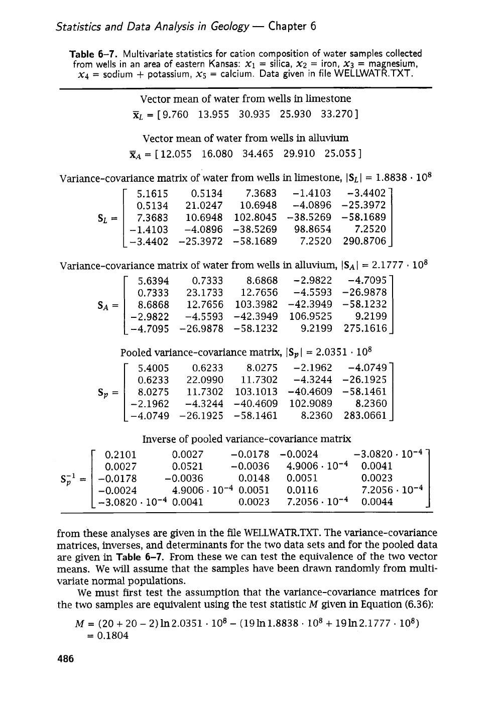
Table
6-7.
Multivariate statistics for cation composition of water samples collected
from wells in an area
of
eastern Kansas:
x1
=
silica,
x2
=
iron,
XJ
=
magnesium,
x4
=
sodium
+
potassium,
xg
=
calcium. Data given in file
WELLWATR.TXT.
Vector mean of water from wells
in
limestone
XL
=
[
9.760 13.955 30.935 25.930 33.2701
Vector mean
of
water from wells in alluvium
XA
=
[
12.055 16.080 34.465 29.910 25.055
]
Variance-covariance matrix
of
water from wells
in
limestone,
ISL
I
=
1.8838
-
lo8
1
1
5.1615
0.5134
7.3683 -1.4103
-3.4402
0.5134
21.0247 10.6948
-4.0896 -25.3972
7.3683
10.6948
102.8045 -38.5269
-58.1689
-1.4103
-4.0896
-38.5269 98.8654
7.2520
-3.4402 -25.3972
-58.1689 7.2520
290.8706
SL=
I
I
Variance-covariance matrix of water from wells
in
alIuvium,
IsAI
=
2.1777
-
lo8
5.6394
0.7333
8.6868 -2.9822
-4.7095
0.7333
23.1733
12.7656 -4.5593
-26.9878
SA
=
8.6868
12.7656 103.3982
-42.3949 -58.1232
-2.9822
-4.5593 -42.3949
106.9525 9.2199
-4.7095
-26.9878 -58.1232
9.2199 275.1616
5.4005
0.6233
8.0275 -2.1962
-4.0749
0.6233
22.0990 11.7302
-4.3244 -26.1925
Sp
=
8.0275
11.7302 103.1013
-40.4609 -58.1461
-2.1962 -4.3244
-40.4609 102.9089
8.2360
I
-4.0749
-26.1925 -58.1461
8.2360 283.0661
Pooled variance-covariance matrix,
ISPI
=
2.0351
lo8
s-1
=
P
Inverse
of
pooled variance-covariance matrix
0.2101 0.0027 -0.0178 -0.0024 -3.0820
-
0.0027 0.0521 -0.0036 4.9006
.
0.0041
-0.0178
-0.0036 0.0148 0.0051
0.0023
-0.0024 4.9006.
lom4
0.0051
0.0116 7.2056
.
-3.0820
lo-*
0.0041 0.0023 7.2056
-
0.0044
from these analyses are given
in
the file WELLWATR.TXT. The variance-covariance
matrices, inverses, and determinants for the two data sets and for the pooled data
are given in
Table
6-7.
From these we can test the equivalence of the
two
vector
means. We will assume that the samples have been drawn randomly from multi-
variate normal populations.
We must first test the assumption that the variance-covariance matrices
for
the two samples are equivalent using the test statistic
M
given
in
Equation
(6.36):
M
=
(20
+
20
-
2)1n2.0351.
lo8
-
(19ln1.8838.
lo8
+
19h2.1777.
lo8)
=
0.1804
486
Analysis
of
Multivariate
Data
The transformation factor,
C-l,
must also be calculated to allow use of the
x2
approximation:
6(5+1)(2-1)
2*52+3*5-1
c-l=
1
-
=
0.8637
The
x2
statistic is approximately
0.1804-0.8637
=
0.1558,
with degrees of freedom
equal to
v
=
1/2(2
-
1)(5)(5
+
1)
=
15.
The critical value of
x2
for
v
=
15
with a
5%
level of significance is
25.00.
The computed statistic is less than this value and does not fall into the critical
region,
so
we may conclude that there is nothing
in
our samples which suggests
that the variance-covariance structures of the parent populations
are
different. We
may pool the two sample variance-covariance matrices and test the equality of the
multivariate means using the
T2
test of Equation
(6.33):
T2
=
-
2o
2o
1.4847
=
14.847
20
+
20
The value
1.4847
is the product of the matrix multiplications
D’Sp’D
specified in
Equation
(6.33).
The
T2
statistic may be converted to
an
F-statistic by Equation
(6.34):
Degrees
of
freedom
are
v1
=
5
and
vz
=
(20
+
20
-
5
-
1)
=
34.
The crit-
ical value for F with
5
and
34
degrees of freedom at the
5%
(a
=
0.05)
level of
signhcance is
2.49.
Our
computed test statistic just exceeds this critical value,
so
we conclude that our samples do, indeed, indicate
a
difference in the means of
the
two
populations. In other words, there is a statistically significant difference
in
composition of water from the two aquifers. This simple test
will
not pinpoint
the chemical variables responsible for this difference, but it does substantiate the
natives’ contention that they
can
tell a difference in the water!
Multivariate techniques equivalent to the analysis-of-variance procedures
discussed in Chapter
2
are
available. In general, these involve a comparison of
two
m
x
m
matrices that
are
the multivariate equivalents of the among-group and
within-group
sums
of squares tested in ordinary analysis of variance. The test
statistic consists of the largest eigenvalue of the matrix resulting from the compari-
son.
We
will not consider these tests here because their formulation is complicated
and their applications to geologic problems have been,
so
far,
minimal. This is
not a reflection on their potential utility, however. Interested readers
are
referred
to chapter
5
of Griffith and Amrhein
(1997),
which presents worked examples of
MANOVA’s
applied to problems in geography. Koch and
Link
(1980)
include a brief
illustration of the application of multivariate analysis of variance to geochemical
data. Statistical details are discussed by Morrison
(1990).
Cluster
Analysis
Cluster analysis is the name given to a bewildering assortment of techniques de-
signed to perform classification by assigning observations to groups
so
each group
is more
or
less homogeneous and distinct from other groups. This is the special
forte of taxonomists, who attempt to deduce the lineage of living creatures from
487
Statistics and Data Analysis in Geology
-
Chapter
6
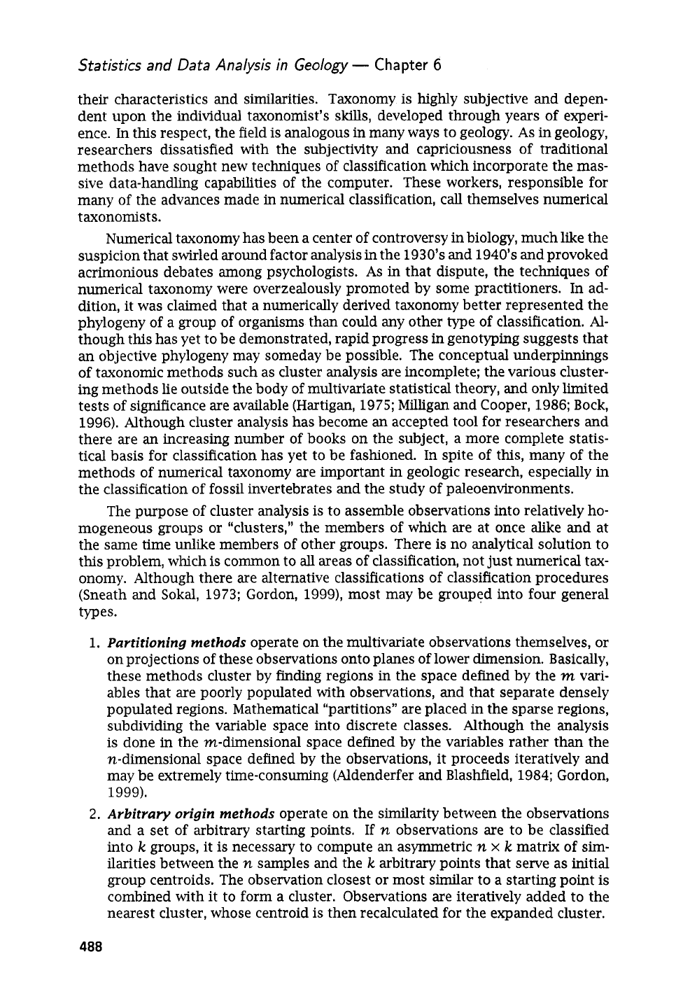
their characteristics and similarities. Taxonomy is highly subjective and depen-
dent upon the individual taxonomist’s
skills,
developed through years of experi-
ence. In this respect, the field is analogous
in
many ways to geology.
As
in geology,
researchers dissatisfied with the subjectivity and capriciousness of traditional
methods have sought new techniques of classification which incorporate the mas-
sive data-handling capabilities of the computer. These workers, responsible for
many of the advances made in numerical classification,
call
themselves numerical
taxonomists.
Numerical taxonomy has been a center of controversy in biology, much like the
suspicion that swirled around factor analysis
in
the 1930’s and 1940’s and provoked
acrimonious debates among psychologists.
As
in that dispute, the techniques of
numerical taxonomy were overzealously promoted by some practitioners.
In
ad-
dition, it was claimed that a numerically derived taxonomy better represented the
phylogeny of a group of organisms than could any other type
of
classification. Al-
though this has yet to be demonstrated, rapid progress in genotyping suggests that
an
objective phylogeny may someday be possible. The conceptual underpinnings
of taxonomic methods such as cluster analysis are incomplete; the various cluster-
ing methods lie outside the body of multivariate statistical theory, and only limited
tests of significance are available (Hartigan, 1975; Milligan and Cooper, 1986; Bock,
1996). Although cluster analysis has become an accepted tool for researchers and
there are
an
increasing number of books on the subject, a more complete statis-
tical basis for classification has yet to be fashioned. In spite
of
this, many of the
methods of numerical taxonomy are important
in
geologic research, especially in
the classification of fossil invertebrates and the study
of
paleoenvironments.
The purpose of cluster analysis is to assemble observations into relatively ho-
mogeneous groups or “clusters,” the members of which are at once alike and at
the same time unlike members of other groups. There is no analytical solution to
this problem, which is common to
all
areas of classification, not just numerical tax-
onomy. Although there are alternative classifications of classification procedures
(Sneath and Sokal, 1973; Gordon, 1999), most may be grouped into four general
types.
1.
Partitioning methods
operate on the multivariate observations themselves, or
on projections of these observations onto planes of lower dimension. Basically,
these methods cluster by finding regions in the space defined by the
m
vari-
ables that are poorly populated with observations, and that separate densely
populated regions. Mathematical “partitions” are placed in the sparse regions,
subdividing the variable space into discrete classes. Although the analysis
is
done in the m-dimensional space defined by the variables rather than the
n-dimensional space defined by the observations, it proceeds iteratively and
may be extremely time-consuming (Aldenderfer and Blashfield, 1984; Gordon,
1999).
2.
Arbitrary origin
methods
operate on the similarity between the observations
and a set of arbitrary starting points.
If
n
observations are to be classified
into
k
groups, it is necessary to compute an asymmetric
n
x
k
matrix of
sim-
ilarities between the
n
samples and the
k
arbitrary points that serve as initial
group centroids. The observation closest or most
similar
to a starting point
is
combined with it to form a cluster. Observations are iteratively added to the
nearest cluster, whose centroid is then recalculated for the expanded cluster.
488
Analysis
of
Multivariate Data
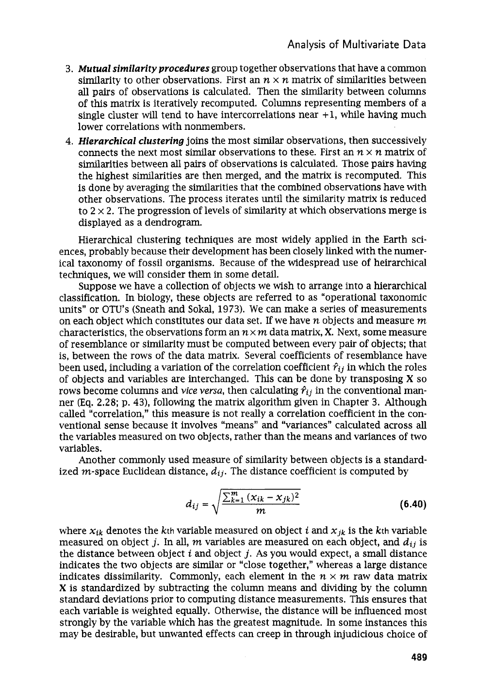
3.
Mutual similarity procedures
group together observations that have a common
similarity to other observations. First an
n
x
n
matrix of similarities between
all pairs
of
observations
is
calculated. Then the similarity between columns
of this matrix is iteratively recomputed. Columns representing members of a
single cluster
will
tend to have intercorrelations
near
+1,
while having much
lower correlations with nonmembers.
4.
Hierarchical clustering
joins the most
similar
observations, then successively
connects the next most similar observations to these. First an
n
x
n
matrix of
similarities between all pairs of observations is calculated. Those pairs having
the highest similarities are then merged, and the matrix is recomputed. This
is
done by averaging the similarities that the combined observations have with
other observations. The process iterates until the similarity matrix is reduced
to
2
x
2.
The progression of levels of similarity at which observations merge
is
displayed as a dendrogram.
Hierarchical clustering techniques are most widely applied
in
the Earth sci-
ences, probably because their development has been closely linked with the numer-
ical taxonomy
of
fossil
organisms. Because of the widespread use of heirarchical
techniques, we will consider them
in
some detail.
Suppose we have a collection of objects we wish to arrange into a hierarchical
classification. In biology, these objects are referred to as “operational taxonomic
units” or
OW’S
(Sneath and Sokal,
1973).
We can make a series of measurements
on each object which constitutes our data set.
If
we have
n
objects and measure
m
characteristics, the observations form an
nx
m
data matrix,
X.
Next, some measure
of resemblance or similarity must be computed between every pair
of
objects; that
is,
between the rows of the data matrix. Several coefficients of resemblance have
been used, including a variation of the correlation coefficient
fij
in which the roles
of objects and variables are interchanged.
This
can
be done by transposing
X
so
rows become columns and
vice
versa,
then calculating
fij
in the conventional man-
ner (Eq.
2.28;
p.
43),
following the matrix algorithm given in Chapter
3.
Although
called “correlation,” this measure
is
not really a correlation coefficient in the con-
ventional sense because it involves “means” and “variances” calculated across
all
the variables measured on two objects, rather than the means and variances of two
variables.
Another commonly used measure
of
similarity between objects is a standard-
ized m-space Euclidean distance,
dij.
The distance coefficient
is
computed by
(6.40)
where
Xik
denotes the
kth
variable measured on object
i
and
xjk
is
the
kth
variable
measured on object
j.
In all,
m
variables are measured on each object, and
dij
is
the distance between object
i
and object
j.
As
you would expect, a small distance
indicates the two objects are similar or “close together,” whereas a large distance
indicates dissimilarity. Commonly, each element in the
n
x
m
raw data matrix
X
is
standardized by subtracting the column means and dividing by the column
standard deviations prior to computing distance measurements.
This
ensures that
each variable
is
weighted equally. Otherwise, the distance will be influenced most
strongly by the variable which has the greatest magnitude.
In
some instances this
may be desirable, but unwanted effects can creep
in
through injudicious choice of
489
Statistics
and
Data
Analysis in
Geology
-
Chapter
6
measurement units.
As
an
extreme example, we might measure three perpendicular
axes on a collection of pebbles.
If
we measure two of the axes in centimeters and the
third
in
millimeters, the third
axis
will
have proportionally ten times more influence
on the distance coefficient than either of the other two variables.
Other measures of similarity that are less commonly used in the Earth sci-
ences include a wide variety of
association coefficients
which are based on binary
(presence-absence) variables or a combination of binary and continuous variables.
The most popular of these are the
simple matching coefficient, Jaccard’s coeffi-
cient,
and
Cower’s coefficient-all
ratios of the presence-absence of properties.
They differ primarily
in
the way that mutual absences (called “negative matches”)
are considered. Sneath and Sokal (1973) discuss the relative merits
of
these
and
other coefficients of association.
Probabilistic similarity coefficients
are used with
binary data and consider the gain or loss of information when objects are combined
into clusters. Again, Sneath and
Sokal(1973)
provide a comprehensive summary.
Computation of a similarity measurement between
all
possible pairs of objects
will
result in
an
n
x
n
symmetrical matrix,
C.
Any coefficient
Cij
in the matrix gives
the resemblance between objects
i
and
j.
The next step is to arrange the objects
into a hierarchy
so
objects with the highest mutual similarity are placed together.
Then groups or clusters
of
objects are associated with other groups which they
most closely resemble, and
so
on until
all
of the objects have been placed into a
complete classification scheme.
Many
variants of clustering have been developed; a
consideration of all of the possible alternative procedures and their relative merits
is
beyond the scope of this book. Rather, we will discuss one simple clustering
technique called the
weighted pair-group method
with
arithmetic averaging,
and
then point out some useful modifications to this scheme.
Extensive discussions of hierarchical and other classification techniques are
contained in books by Jardine and Sibson (1971), Sneath and Sokal (1973),
Har-
tigan (19751, Aldenderfer and Blashfield (1984), Romesburg (1984), Kaufman
and
Rousseeuw (1990), Backer (1995), and Gordon (1999). Diskettes containing cluster-
ing programs are included in some of the these books or are available separately at
modest cost.
In
addition, most personal computer programs for statistical analysis
contain modules for hierarchical clustering.
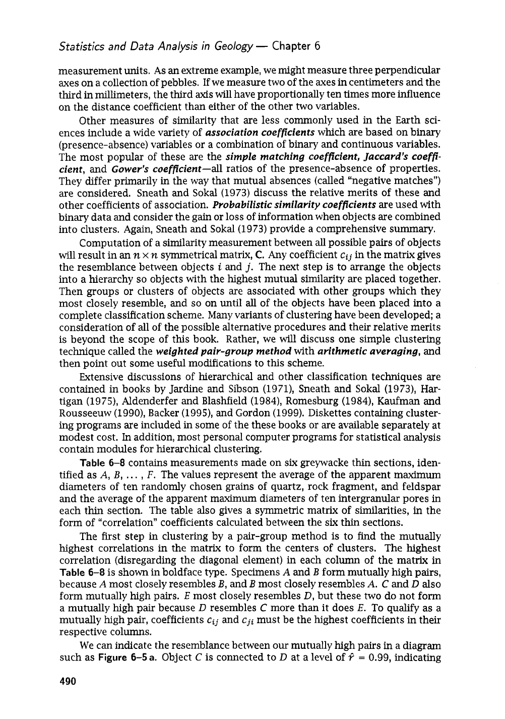
Table
6-8
contains measurements made on
six
greywacke thin sections, iden-
tified as
A,
B,
.
. .
,
F.
The values represent the average of the apparent maximum
diameters of ten randomly chosen grains of quartz, rock fragment, and feldspar
and the average of the apparent maximum diameters of ten intergranular pores in
each thin section. The table also gives
a
symmetric matrix of similarities,
in
the
form of “correlation” coefficients calculated between the
six
thin sections.
The first step in clustering by a pair-group method is to find the mutually
highest correlations in the matrix to form the centers of clusters. The highest
correlation (disregarding the diagonal element) in each column of the matrix
in
Table
6-8
is shown in boldface type. Specimens
A
and
B
form mutually high pairs,
because
A
most closely resembles
B,
and
B
most closely resembles
A.
C
and
D
also
form mutually high pairs.
E
most closely resembles
D,
but these two do not form
a mutually high pair because
D
resembles
C
more than it does
E.
To qualify as a
mutually high pair, coefficients
Cij
and
Cji
must be the highest coefficients in their
respective columns.
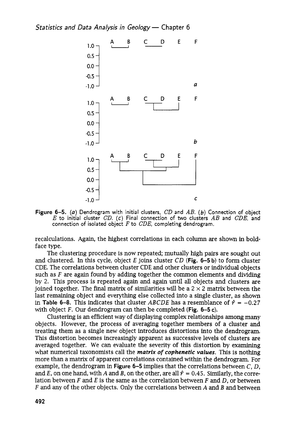
We can indicate the resemblance between our mutually high pairs in a diagram
such as
Figure
6-5
a.
Object
C
is connected to
D
at a level of?
=
0.99, indicating
490
Analysis
of
Multivariate Data
Table
6-8.
Average apparent grain diameters measured on thin sections of six
greywackes and matrix of “correlations” between thin sections. Highest
“correlation” in each column
is
indicated in boldface type.
Average diameters
in
mm
Rock frag-
Specimen
Pore Quartz
ment Feldspar
A
0.24
1.78 0.69
3.32
B
0.48
2.07
2.41 4.78
C
0.76 4.05
1.2
3.21
D
0.23
2.98 0.85 2.06
E
0.04
3.33
3.39 2.63
F
1.98
0.98
2.01 2.02
“Correlations” on
initial
iteration
A
B
C
D
E
F
A
1
0,9110
0.7671 0.7041
0.4401 -0.1067
B
0.91
10
1
0.5393
0.4996 0.5704
0.1680
C
0.7671 0.5393
1
0.9910
0.5873 -0.7187
D
0.7041 0.4996
0.9910
1
0.6647
-0.7675
E
0.4401
0.5704 0.5873
0.6647
1
-0.3883
F
-0.1067
0.168 -0.7187 -0.7675
-0.3883
1
“Correlations” on second iteration
AB
CD
E
F
AB
1
0.394
0.505
0.031
CD
0.394
1
0.626
-0.744
E
0.505
0.626
1
-0.388
F
0.031 -0.744 -0.388
1
“Correlations” on third iteration
AB
CDE
F
AB
1
0.450
0.031
CDE
0.450
1
-0.566
F
0.031 -0.566
1
“Correlations”
on
fourth iteration
ABCDE
F
ABCDE
1
-0.268
F
-0.268
1
the degree of their mutual similarity.
In
the same manner,
A
and
B
are connected
at a level
of
Q
=
0.91.
This
is the first step in the construction
of
a
dendrogrum,
or
tree diagram, which
is
the most common way
of
displaying the results of clustering.
Next, the similarity matrix must be recomputed, treating grouped or clustered
elements as a single element.
There are several methods for doing this. In the
simple technique we
are
considering, new correlations between
all
clusters and
unclustered objects are recalculated by simple arithmetic averaging. For exam-
ple, the new correlation between cluster
CD
and object
E
is equal to the
sum
of
the correlations of the elements collZmon to both
CD
and
E,
divided by
2
(that
is,
Q
=
(0.5873
+
0.6647)/2
=
0.626).
Table
6-8
contains the results
of
these
491
Statistics and Data Analysis in Geology
-
Chapter
6
-0.5
-1
.o
1
.o
-0.5
-1
.o
-0.5
-1
.o
ABCDEF
U
a
ABCDEF
TI
U
b
ABCDEF
C
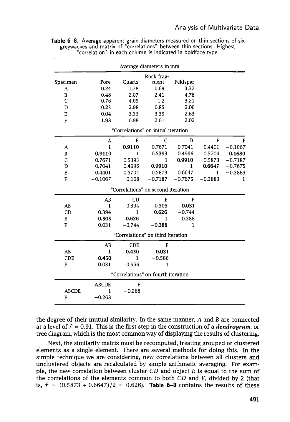
Figure
6-5.
(a)
Dendrogram with initial clusters,
CD
and
AB.
(b)
Connection
of
object
E
to initial cluster
CD.
(c)
Final connection
of
two
clusters
AB
and
CDE,
and
connection
of
isolated object
F
to
CDE,
completing dendrogram.
recalculations. Again, the highest correlations in each column are shown in bold-
face type.
The clustering procedure
is
now repeated; mutually high pairs are sought out
and clustered. In this cycle, object
E
joins cluster
CD
(Fig.
6-5
b)
to form cluster
CDE.
The correlations between cluster
CDE
and other clusters or individual objects
such as
F
are again found by adding together the common elements and dividing
by
2.
This process
is
repeated again and again until
all
objects
and
clusters are
joined together. The
final
matrix of similarities
will
be a
2
x
2
matrix between the
last remaining object and everything else collected into a single cluster, as shown
in
Table
6-8.
This indicates that cluster
ABCDE
has a resemblance of?
=
-0.27
with object
F.
Our
dendrogram can then be completed
(Fig.
6-5
c).
Clustering is
an
efficient way of displaying complex relationships among many
objects. However, the process of averaging together members of a cluster and
treating them as a single new object introduces distortions into the dendrogram.
This distortion becomes increasingly apparent as successive levels of clusters are
averaged together. We can evaluate the severity
of
this distortion by examining
what numerical taxonomists call the
matrix
of
cophenetic values.
This is nothing
more than a matrix of apparent correlations contained within the dendrogram. For
example, the dendrogram in
Figure
6-5
implies that the correlations between
C,
D,
and
E,
on one hand, with
A
and
B,
on the other, are
all
?
=
0.45.
Similarly, the corre-
lation between
F
and
E
is the same as the correlation between
F
and
D,
or between
F
and
any of the other objects. Only the correlations between
A
and
B
and between
492
Next Page
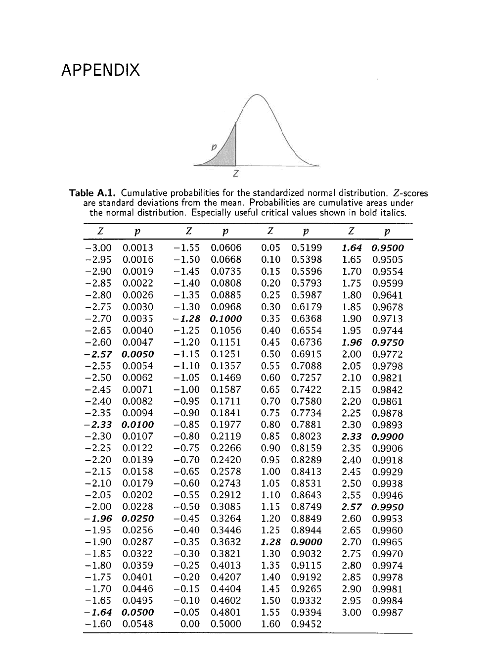
APPENDIX
Table
A.l.
Cumulative probabilities for the standardized normal distribution. Z-scores
the normal distribution. Especially useful critical values shown in bold italics.
are standard deviations from the mean. Probabilities are cumulative areas under
Z
P
Z
P
Z
P
Z
P
-3.00 0.0013
-2.95 0.0016
-2.90 0.0019
-2.85
0.0022
-2.80 0.0026
-2.75 0.0030
-2.70 0.0035
-2.65 0.0040
-2.60 0.0047
-2.57 0.0050
-2.55
0.0054
-2.50 0.0062
-2.45 0.0071
-2.40 0.0082
-2.35 0.0094
-2.33 0.0100
-2.30 0.0107
-2.25 0.0122
-2.20 0.0139
-2.15
0.0158
-2.10 0.0179
-2.05 0.0202
-2.00 0.0228
-1.96 0.0250
-1.95 0.0256
-1.90 0.0287
-1.85 0.0322
-1.80 0.0359
-1.75 0.0401
-1.70 0.0446
-1.65 0.0495
-1.64 0.0500
-1.60 0.0548
-1.55
0.0606
-1.50 0.0668
-1.45 0.0735
-1.40 0.0808
-1.35
0.0885
-1.30 0.0968
-1.28 0.1000
-1.25
0.1056
-1.20 0.1151
-1.15 0.1251
-1.10 0.1357
-1.05 0.1469
-1.00 0.1587
-0.95 0.1711
-0.90 0.1841
-0.85 0.1977
-0.80 0.2119
-0.75 0.2266
-0.70 0.2420
-0.65 0.2578
-0.60 0.2743
-0.55
0.2912
-0.50 0.3085
-0.45 0.3264
-0.40 0.3446
-0.35 0.3632
-0.30 0.3821
-0.25 0.4013
-0.20 0.4207
-0.15 0.4404
-0.10 0.4602
-0.05 0.4801
0.00
0.5000
0.05 0.5199
0.10 0.5398
0.15 0.5596
0.20 0.5793
0.25 0.5987
0.30 0.6179
0.35 0.6368
0.40 0.6554
0.45 0.6736
0.50 0.6915
0.55
0.7088
0.60 0.7257
0.65 0.7422
0.70 0.7580
0.75 0.7734
0.80 0.7881
0.85 0.8023
0.90 0.8159
0.95 0.8289
1.00 0.8413
1.05 0.8531
1.10 0.8643
1.15
0.8749
1.20 0.8849
1.25
0.8944
1.28 0.9000
1.30 0.9032
1.35
0.9115
1.40 0.9192
1.45 0.9265
1.50 0.9332
1.55
0.9394
1.60 0.9452
1.64 0.9500
1.65 0.9505
1.70 0.9554
1.75 0.9599
1.80 0.9641
1.85 0.9678
1.90 0.9713
1.95 0.9744
1.96 0.9750
2.00 0.9772
2.05 0.9798
2.10 0.9821
2.15
0.9842
2.20 0.9861
2.25
0.9878
2.30 0.9893
2.33
0.9900
2.35 0.9906
2.40 0.9918
2.45 0.9929
2.50 0.9938
2.55
0.9946
2.57 0.9950
2.60 0.9953
2.65 0.9960
2.70 0.9965
2.75 0.9970
2.80 0.9974
2.85 0.9978
2.90 0.9981
2.95 0.9984
3.00 0.9987