Daniels M.J., Hogan J.W. Missing Data in Longitudinal Studies: Strategies for Bayesian Modeling and Sensitivity Analysis

Подождите немного. Документ загружается.

60 BAYESIAN INFERENCE

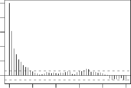
01020304050

0.0 0.2 0.4 0.6 0.8 1.0

Lag

ACF

Figure 3.2 Autocorrelation plot. Lag-k correlation is plotted vs. k.

of the chain into m batches of length m



,suchthat m



is large enough for

the correlation between batch means to be negligible. To calculate the pos-

terior variance, we use a suitably normalized corrected sum of squares of the

batchmeans (see pp. 194–195 in Carlin and Louis, 2000). Other approaches,

including some based on time series methodology, can be found in Chapter 5

of Carlin and Louis (2000).

Marginal posterior distributions

The MCMC sample obtained provides a (dependent) sample from the joint

posterior distribution of interest. However, we are often interested in marginal

posterior distributions; for example, in the multivariate normal model in Ex-

ample 2.3, we may be interested in a speciﬁc regression coeﬃcient, say β

sample from the marginal posterior distribution of β

(or, in general, any func-

tion of the parameters) is obtained by using only the sampled values of that

parameter. To obtain the marginal posterior distribution for a function of the

parameters, we can evaluate that function at each iteration, given the current

values of the parameters, to obtain a sample from the marginal posterior of

that function. See Section 4.4 for an illustration.

COMPUTATION OF THE POSTERIOR DISTRIBUTION 61

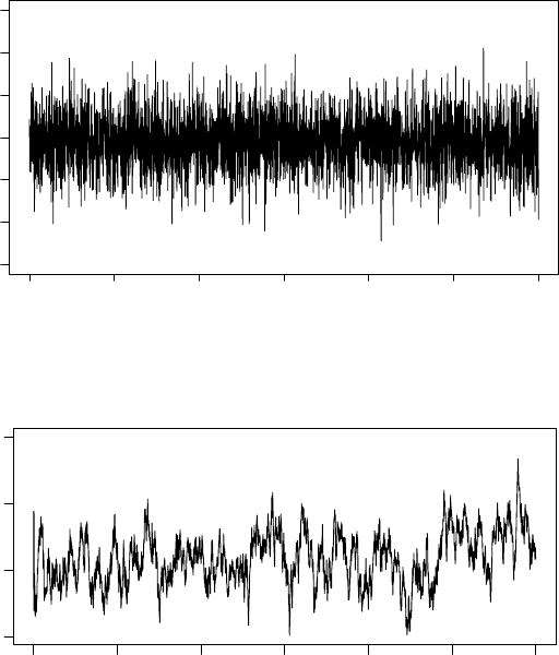
0 500 1000 1500 2000 2500 3000

−10 0 10 20304050

iteration

beta

0 500 1000 1500 2000 2500 3000

25 30 35 40

iteration

beta

Figure 3.3 Plot illustrating good mixing (top) and poor mixing (bottom).

Reweighting

It will sometimes be the case that we have a sample from a distribution

(e.g., an MCMC sample from the posterior) and we would like to use this

sample to make inference based on a similar posterior (maybe with a slightly

diﬀerent likelihood and/or priors). We can avoid re-running a Gibbs sampler

on this new model by appropriately reweighting the sample already obtained.

In general, suppose we have a sample from some distribution, p(θ)andwe

want to make inferencebasedon some diﬀerent distribution, p



(θ). Then, we

62 BAYESIAN INFERENCE

can reweight the sample using weights of the form

w =

p(θ)



(θ)

The reliability of this approach depends on the weights, w being stable (Pe-

ruggia, 1997). Reweighting will be useful for computing intractable likelihoods

(e.g., the multivariate probit model in Example 2.6) that are sometimes needed

for model selection criterion (see Section 3.5)andforcomputing several model

selection criteria in the presence of incomplete data (see Chapters 6 and 8).

Anoteonimproperpriors and Gibbs sampling

We end this section on posterior sampling with a cautionary remark on using

improper priors in Gibbs sampling (Hobert and Casella, 1996), illustrated

by an example. Consider the normal random eﬀects model in Example 2.1.

Suppose we specify the following (improper) prior on Ω,

p(Ω) ∝|Ω|

−(p+1)/2

where p =dim(Ω). Clearly,



p(Ω) dΩ = ∞.

The full conditional distribution of Ω

−1

will be a proper Wishart distri-

bution. However, the posterior distribution of Ω

−1

will be improper.This

phenomenon (when using improper priors) of all the full conditionals being

proper distributions, but the posterior being improper, was ﬁrst noticed in

Hobert and Casella (1996). An even more problematic aspect from a practical

perspective is that the sample from the improper posterior may not indicate

any problems! So, when using improper priors, the propriety of the poste-

rior distribution needs to be veriﬁed analytically. Otherwise, improper priors

should not be used. If WinBUGS is being used, this is not a concern as it does

not allow improper priors; however, for investigators writing their own code

and using improper priors, this is an important issue.

3.5 Model comparisons and assessing model ﬁt

When we ﬁt a parametric model to a dataset, we should examine how well

the model ﬁts the observed data. A related issue is how to select among sev-

eral plausible models (model selection), which tells us only about the ﬁt of

models relative to the others under consideration. We address model selec-

tion ﬁrst. Two common criteria are the deviance information criterion (DIC)

(Spiegelhalter et al., 2002) and posterior predictive loss (PPL) (Gelfand and

Ghosh, 1998). Both take into account goodness of ﬁt while penalizing models

for overﬁtting (a complexity penalty).

MODEL FIT 63

3.5.1 Deviance Information Criterion (DIC)

The DIC is a model-based criterion composed of a goodness of ﬁt term and

apenaltyterm.Theﬁt is measured by the deviance, a linear function of the

log likelihood, given by

Dev(θ)=−2logL(θ | y).

Larger values of the deviance indicate poorer ﬁt.

The penalty term measures model complexity and is given by

= E{Dev(θ) | y}−Dev{E(θ | y)}. (3.10)

The variable p

is called the eﬀective number of parameters. As the variability

in the posterior of θ decreases, p

→ 0. How overﬁtting is penalized can best

be understood by introducing the concept of the residual information in data

y conditional on parameters θ,deﬁned as −2log{p(y | θ)} (Kullback and

Liebler, 1951; Burham and Anderson, 1998). Recall that L(θ | y) ∝ p(y | θ).

Deﬁne



θ to be an estimator of θ and θ



to be the true parameter value. The

diﬀerence between the residual information at the true parameter value and

at the estimated parameter value is

−2logp(y | θ



)+2logp(y |



θ). (3.11)

This can be interpreted as the degree of overﬁtting due to the inﬂuence of y

on the estimator



θ.InaBayesiananalysis, θ is random and we can replace

(3.11) with its posterior expectation, the eﬀective number of parameters p

given in (3.10).

The DIC itself is deﬁned as

DIC = Dev{E(θ | y)} +2p

. (3.12)

The ﬁrst term measures goodness of ﬁt and the second term is the complexity

penalty. The form is very similar to the Akaike Information Criterion (AIC)

(Akaike, 1973). Equivalently, the DIC can be written explicitly as a function

of the log likelihood,

DIC = −4E{log L(θ | y) | y} +2logL{E(θ | y) | y}, (3.13)

which will be a more convenient form for its development in thesetting of

incomplete data and for describing its computation in Chapters 6 and 8.

The DIC is easy to compute from a posterior sample; it requires calculat-

ing two quantities, E{Dev(θ) | y} and Dev{E(θ | y)},usingtheoutput from

MCMC approaches; WinBUGS will often calculate it automatically. Ease of

implementation has contributed to itswidespread use. In Section 4.2, we use

the DIC to compare several multivariate normal models for the Growth Hor-

mone data (described in Section 1.3)

An advantage of the DIC over approaches like AIC, where the user speciﬁes

the number of parameters, is that the (eﬀective) number of parameters is

64 BAYESIAN INFERENCE

counted automatically (see (3.10)). This is particularly helpful in multilevel

models where the number of parameters is sometimes diﬃcult to quantify. As

an example, consider the normal random eﬀects models in Example 2.1 with

likelihood given by

L(θ, b

| y) ∝



i=1

|Σ|

−1/2

exp



−

(β, b

)

−1

(β, b

)



, (3.14)

where e

(β, b

)=y

− x

β − w

and θ =(β, Σ). The random eﬀects have

not been integrated out and are now treated as parameters along with θ.On

the surface, if we count the number of random eﬀects (assume for simplicity

they are one-dimensional), there are n.However, the eﬀective number can be

quite smaller because the random eﬀects distribution p(b

| θ)shrinksthe

random eﬀects to zero. As the variance of the random eﬀects distribution

goes to zero, there are fewer parameters; in fact, if the variance is zero, all the

random eﬀects are identically zero so there are in fact no parameters. On the

other hand, as the varianceincreases,the number of parameters approaches n.

Despite its computational simplicity, the DIC does have drawbacks. The

best model as determined by the DIC can change depending on the choice of

‘likelihood’ (see Trevisani and Gelfand, 2003); for example, again revisiting

the normal random eﬀects model (Example 2.1), the likelihood can take one

of two forms: the integrated likelihood given in (3.2), or the likelihood without

the random eﬀects integrated out, given in (3.14).

In addition, the DIC is not invariant to the parameterization of θ.Thisoc-

curs because the ﬁt term Dev{E(θ | y)} in (3.12) involves a plug-in estimator

for θ based on the posterior, E(θ | y); and ingeneral, E{h(θ) | y} = h{E(θ |

y)}.Forthemultivariate normal model in Example 2.3, θ could be deﬁned

as (β, Σ

−1

)or(β, Σ). Using Σ vs. Σ

−1

will result in diﬀerent values for the

DIC; see Section 4.2 for an illustration on the Growth Hormone data. For

covariance matrices, Spiegelhalter et al. (2002) recommend using the inverse

because its posterior mean is more stable.

Another limitation, common to all likelihood based criteria, is that for some

models, the likelihood is not available in closed form (e.g., the multivariate

probit model in Example 2.6). For many models, to evaluate the likelihood,

it is possible to use Monte Carlo integration and reweighting. For example, in

the multivariate probit model, we need to compute







j=1

I{z

> 0}

I{z

< 0}

1−y





given (β, Σ), where z

follows a multivariate normal distribution with mean

β and covariance matrix Σ.Wecansamplefrom the distribution of z

and

compute the expectation by averaging the term in brackets over the samples.

MODEL FIT 65

However, it would be computationally prohibitive to do this for every sampled

value of θ =(β, Σ)thatisneeded to compute E{Dev(θ)} in the DIC.

Amorepractical approach is reweighting (as discussed in Section 3.4.4). To

implement it here, we can take a likely value, say θ



= E(θ | y), and sample

L values, z

(l)

: l =1,...,L,fromZ

∼ N(x



, Σ



), where θ



=(β



, Σ



Then, to compute the likelihood for other values of θ,weevaluate



h(z

(l)



where h(z)=

I(z

> 0)

I(z

< 0)

1−y

.Theweightsaregivenby

p(z

(l)

| θ)

p(z

(l)

| θ



)

where p(·|θ)isamultivariate normal distribution with parameters θ =

(β, Σ)(Liu and Daniels, 2007). We illustrate this in Section 7.5. For further

recommendations and discussion on the choice of likelihood and parameteri-

zation, we refer the reader to Spiegelhalter et al. (2002).

3.5.2 Posterior predictive loss

Posterior predictive loss (PPL) (Gelfand and Ghosh, 1998) is another model

selection criterion. Before providing details, we ﬁrst need to deﬁne the poste-

rior predictive distribution.

Deﬁnition 3.6. Posterior predictive distribution.

The posterior predictive distribution is

p(y

rep

| y)=



p(y

rep

| θ, y)p(θ | y)dθ, (3.15)

where p(y

rep

| θ, y)=p(y

rep

| θ). Samples from the posterior predictive

distribution are replicates of the observed data generated by the model. 2

PPL quantiﬁes the ﬁt of the model by comparing features of the (model-

based) posterior predictive distribution to equivalent features of the observed

data. The comparison is based on a user-chosen loss function. L (y

rep

,a; y),

where a is chosen to minimize the expectation of the loss with respect to

the posterior predictive distribution E{L (y

rep

,a; y) | y}, i.e., the posterior

predictive loss. For some choices of L ,theminimization has a closed form.

Gelfand and Ghosh consider lossfunctions of the form

rep

,a; y)=L (y

rep

,a)+kL (y,a),k≥ 0. (3.16)

66 BAYESIAN INFERENCE

For univariate y,ifL is chosen as squared error loss, it can be shown that

min



rep

,a; y) | y





i=1

k +1



i=1

(µ

− y

)

= P +

k +1

G, (3.17)

where

= E(Y

i,rep

| y)=



i,rep

p(y

i,rep

| θ) p(θ | y) dθ dy

i,rep

is the posterior predictive mean and σ

=var(Y

i,rep

| y)istheposterior

predictive variance.

The ﬁrst termin(3.17), P =



i=1

,isapenaltyterm.Overﬁtting the

model will result in large predictive variances σ

and a large value for P .The

second term, G =



i=1

(µ

−y

)

,isagoodness of ﬁt term, which will decrease

with model complexity. This statistic is easy to compute using samples from

the posterior predictive distribution.

For other (smooth) choices of L (·), the criterion can also be approximated

in a similar form with a goodness of ﬁt and a complexity term. Like the DIC,

this criterion contains an ‘automatic’ penalty P .Thechoice of k determines

how much weight is placed on the goodness of ﬁt term relative to the penalty

term. As k →∞, k/(k +1)→ 1. Unlike the DIC, which uses a non-invariant

plug-in estimator for θ, PPL is based ontheposteriorpredictivedistribution

and is invariant to the model parameterization.

The downsides of PPL are that it requiresthechoiceof an appropriate loss

function (which we do not specify in the course of most Bayesian analyses)

and possibly nontrivial analytical calculations to obtain the criterion. Another

issue is applying it to multivariate observations (e.g., longitudinal data), where

we have to account for correlation when computing both the penalty and the

ﬁt terms. However, approaches such as using the log likelihood loss can account

forcorrelation (Gelfand and Ghosh, 1998). Finally, extensions of this criterion

to incomplete data are an area that needs further study.

Asimplewaytoextend this approach to longitudinal (correlated) data,

without using a loss function based on the likelihood, is to summarize each

multivariate observation with a univariate measure T

= h(Y

), which is a

function of the response vector for subject i,andthenapply univariate meth-

ods(Hogan and Wang, 2001). The univariate summary T

might be speciﬁed

as a weighted average of the longitudinal responses, T



for some

ﬁxed set of weights. To emphasize ﬁt based on the last observation time, we

can set



0 l =1,...,J − 1

1 l = J.

MODEL FIT 67

When emphasis is on a change from baseline, set











0 l =2,...,J − 1

1 l =1

−1 l = J.

Given the choice of T

and using the Gelfand and Ghosh loss function (3.16)

with squared error loss, the PPL criterion becomes

PPL =



i=1

i(T )

k +1



i=1

(µ

i(T )

− T

)

(3.18)

= P +

k +1

where µ

i(T )

= E(T

i,rep

| y)andσ

i(T )

=var(T

i,rep

| y), with T

i,rep

= h(Y

i,rep

In Section 4.4, we illustrate this approach on the CTQ I smoking cessation

data (described in Section 1.4).

3.5.3 Posterior predictive checks

To determine how well the model ﬁts the data in an absolute sense, posterior

predictive checks can be used. They are a simple but versatile approach to

determine whether particular aspects of the data are captured adequately by

the model. They require sampling from the posterior predictive distribution

given in (3.15). The draws from p(y

rep

| y)canbemade using the MCMC

output. In particular, for each draw of θ from the MCMCsample,wesample

asetofreplicated data from p(y

rep

| θ). This is easy to do in WinBUGS.

Model critique requires choosing an appropriate data summary T ,which

may be a function of the parameters θ,andcomparingits value based on

the observed data, T (y

obs

; θ), to its values based on the replicated data,

T (y

rep

; θ). We provide some examples relevant for longitudinal data next.

Gelman, Meng, and Stern (1996) proposed Pearson’s χ

statistics as an

overall measure of model ﬁt (designed for independent data). For (temporally

aligned) longitudinal data, we might use a multivariate version

T (y; θ)=



i=1

(θ), (3.19)

where

(θ)={y

− E(y

| θ)}

Σ(θ)

−1

− E(y

| θ)} (3.20)

and Σ(θ)=var(Y

| θ). Another global measure is the empirical distribution,



F of Q

(θ),

T (y; θ)={



F }. (3.21)

68 BAYESIAN INFERENCE

The distribution of residuals for each time point,

(θ)=

− E(Y

| θ)

var(Y

| θ)

1/2

might also be considered. Numerous other summaries can be chosen based on

the application.

Posterior predictive probabilities are a means of quantifying the relationship

between the statistics computed based on the observed data and the statistics

computed based on the replicated data, and can be used to assess model ﬁt.

Deﬁnition 3.7. Posterior predictive probability.

The posterior predictive probability based on data summary T (·; θ)isdeﬁned





h(T (y

obs

; θ), T (y

rep

; θ)) >c



p(y

rep

| θ, y) p(θ | y) dθ dy

rep

for some function h(·)andconstant c. 2

For the multivariate version of Pearson’s χ

(3.19), we might set c =0and

h{T (y

obs

; θ),T(y

rep

; θ)} = T (y

obs

; θ) − T (y

rep

; θ).

Forthe empirical cdf (3.21), we might again set c =0and

h{T (y

obs

; θ), T (y

rep

; θ)} =sign× arg max



obs

(x) −



rep

(x)}|, (3.22)

where



obs

(x)istheempirical cdf of Q

(θ)based on y

obs



rep

(x)isthe

empirical cdf of Q

(θ)based on y

rep

,andsignisthe sign of this maximum

deviation. Extreme probabilities, either close to 0 or close to 1, suggest lack

of ﬁt with respect to T (·; θ).

We illustrate these checks in our analyses of the Growth Hormone data in

Section 4.2. We discuss modiﬁcations to these checks for incomplete data in

Chapters 6and8.

3.6 Nonparametric Bayes

Nonparametric and semiparametric Bayesian approaches that weaken model

assumptions have become much more common in the literature in recent years

due to breakthroughs in computations. In the context of semiparametric re-

gression, we have discussed spline approaches to model a trajectory over time

nonparametrically in Examples 2.7 and Example 3.10. There are also a variety

of approaches (see Further Reading) to specify distributions on the responses

or random eﬀects nonparametrically. Here we focus on mixtures of Dirichlet

process models (Escobar, 1994; MacEachern, 1994) as a way to do this. This

approach can often be implemented in WinBUGS (see Section 10.4 where it

is used to specify the dropout distribution).

Consider univariate responses y

with distribution p(y

| θ

). Assume the