Dan B. Marghitu, Mechanisms and Robots Analysis with MATLAB®
Подождите немного. Документ загружается.

4.6 Slider-Crank (R-RRT) Mechanism 135
eqM2 = cross(rB-rC2,F12)+cross(rC-rC2,F32)+Min2;
eqM2z = eqM2(3);
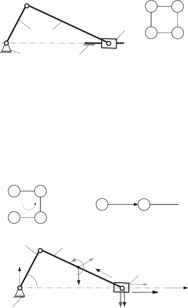
For the crank 1 (Fig. 4.18), there are two vectorial equations
∑
F
(1)
= F
21
+ F
in1
+ G
1
+ F
01
= 0,
∑
M
(1)
A
= r
B
×F
21
+ r
C
1
×(F
in1
+ G
1
)+M
in1
+ M = 0,
where M = |M| is the magnitude of the input moment on the crank, F
21
= −F
12
,
and F
01
= F
01x
ı + F
01y
j.
The above vectorial equations give three scalar equations on x, y, and z
∑
F
(1)
·ı = F
21x
+(−m
1
a
C
1x
)+F
01x
= 0,
∑
F
(1)
·j = F
21y
+(−m
1
a
C
1y
) −m
1
g + F
01y
= 0,
ıj
k
x
B
y
B
0
F
21x
F
21y
0
+
ıj
k
x
C
1
y
C
1
0
−m
1
a
C
1x
−m
1
a
C
1y
−m
1
g 0
−I
C
1
α
1
k + M k = 0,
or
F
21x
+(−m
1
a
C
1x
)+F
01x
= 0,
F
21y
+(−m
1
a
C
1y
) −m
1
g + F
01y
= 0,
x
B
F
21y
−y
B
F
21x
+ x
C
1
(−m
1
a
C
1y
−m
1
g) −y
C
1
(−m
1
a
C
1x
) −I
C
1
α
1
+ M = 0,
F
in 1
= −m
1
a
C
1
M
in 1
= −I
C1
α
1
D’ALEMBERT
F
(1)
= F
21
+ F
in 1
+ G
1
+ F
01
= 0
M
(1)
A
= r
B
× F
21
+ r
C1
× (F
in 1
+ G
1
)+M
in 1
+ M = 0
1
A
M
B
C
1
F
21
F
01
F
21y
F
21x
F
in 1
M
in 1
F
01y
G
1
F
01x
Fig. 4.18 D’Alembert’s principle for link 1
136 4 Dynamic Force Analysis
or numerically
1
4
(400 + 7
√
2)+
−1(−
√
2
4
)
+ F
01x
= 0, (4.43)
−
5
4
(84 +
√
2)+
−1(−
√
2
4
)
−1(10)+F
01y
= 0, (4.44)
√
2
2
−
5
4
(84 +
√
2)
−
√
2
2
1
4
(400 + 7
√
2)
+
√
2
4
−1(−
√
2
4
) −1(10)
−
√
2
4
−1(−
√
2
4
)
−0 + M = 0. (4.45)
For the crank 1 the MATLAB commands are:
F01 = [ sym(’F01x’,’real’) sym(’F01y’,’real’) 0 ];
Mm=[00sym(’Mmz’,’real’) ];
eqF1 = F01+Fin1+G1-F12;
eqF1x = eqF1(1);
eqF1y = eqF1(2);
eqM1 = cross(rB-rC1,-F12)+cross(rA-rC1,F01)+Min1+Mm;
eqM1z = eqM1(3);
Equations 4.38–4.45 form a system of 8 equations with eight scalar unknowns.
The MATLAB commands for solving the system of equations are:
sol321 = solve(eqF3x,eqF3y,eqF2x,eqF2y,eqM2z,...
eqF1x,eqF1y,eqM1z);
F03ys = eval(sol321.F03y);
F23xs = eval(sol321.F23x);
F23ys = eval(sol321.F23y);
F12xs = eval(sol321.F12x);
F12ys = eval(sol321.F12y);
F01xs = eval(sol321.F01x);
F01ys = eval(sol321.F01y);
Mmzs = eval(sol321.Mmz);
The following numerical solutions are obtained
F
03y
= −85 −
3
√
2
2
N,
F
23x
= −100 −
√
2N, F
23y
= 95 +
3
√
2
2
N,
4.6 Slider-Crank (R-RRT) Mechanism 137
F
12x
= −
1
4
(400 + 7
√
2) N, F
12y
=
5
4
(84 +
√
2) N,
F
01x
= −2(50 +
√
2) N, F
01y
= 115 +
√
2N,
M = 3 + 105
√
2Nm.
The MATLAB program using D’Alembert principle and the results are given in
Appendix C.2.
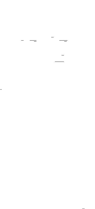
4.6.2.3 Dyad Method
B
R
C
R
C
T
Dyad
Figure 4.19 shows the dyad B
R
C
R
C
T
with the unknown joint reactions F
12
and
F
03
. The joint reaction F
03
is perpendicular to the sliding direction F
03
⊥ Δ = ı or
F
03
= F
03y
j. The following equations are written to determine F
12
and F
03
• Newton’s equation for links 2 and 3,
∑
F
(2&3)
=⇒
m
2
a
C
2
+ m
3
a
C
3
= F
12
+ G
2
+ G
3
+ F
03
+ F
ext
,
or
m
2
a
C
2x
+ m
3
a
C
3x
= F
12x
+ F
ext
,
m
2
a
C
2y
+ m
3
a
C
3y
= F
12y
−m
2
g −m
3
g + F
03y
−m
2
a
C
2y
,
or
B
2
3
C
2
C
F
12
G
3
F
03
G
2
F
12x
F
12y
2
3
C
2
C
Dyad RRT
B
m
2
a
C
2
I
C2
α
2
m
3
a
C
3
NEWTON-EULER
Free-Body Diagram (FBD)
F
ext
(Kinetic Diagram)
Fig. 4.19 Newton–Euler diagrams for dyad B
R
C
R
C
T

138 4 Dynamic Force Analysis
F
12x
+ 102.475 = 0, (4.46)
F
12y
+ F
03y
−19.6464 = 0. (4.47)
• Euler equation of moments for links 2 about C
R
,
∑
M
(2)
C
=⇒
I
C
2
α
2
+ r
CC
2
×m
2
a
C
2
= r
CB
×F
12
+ r
CC
2
×G
2
,
or
−0.707105F
12y
−0.707105F
12x
+ 3.03552 = 0. (4.48)
Equations 4.46–4.48 give
F
12x
= −102.475 N, F
12y
= 106.768 N, and F
03y
= −87.1213 N.
The joint reaction force F
32
is calculated from
F
32
= m
2
a
C
2
−(G
2
+ F
12
)=101.414ı −97.1213 j N.
The MATLAB commands for finding the unknowns using the dyad method are:
F03=[0sym(’F03y’,’real’) 0 ];
F12 = [ sym(’F12x’,’real’) sym(’F12y’,’real’) 0 ];
eqF23 = F03+Fe+G3+F12+G2-m3
*
aC3-m2
*
aC2;
eqF32x = eqF32(1);
eqF32y = eqF32(2);
eqM2C = cross(rB-rC,F12)+cross(rC2-rC,G2)-...
IC2
*
alpha20-cross(rC2-rC,m2
*
aC2);
eqM2Cz = eqM2C(3);
sol32=solve(eqF32x,eqF32y,eqM2Cz);
F03ys=eval(sol32.F03y);
F12xs=eval(sol32.F12x);
F12ys=eval(sol32.F12y);
F03s=[0,F03ys, 0 ];
F12s = [ F12xs, F12ys, 0 ];
F32=m2
*
aC2-(F12s+G2);
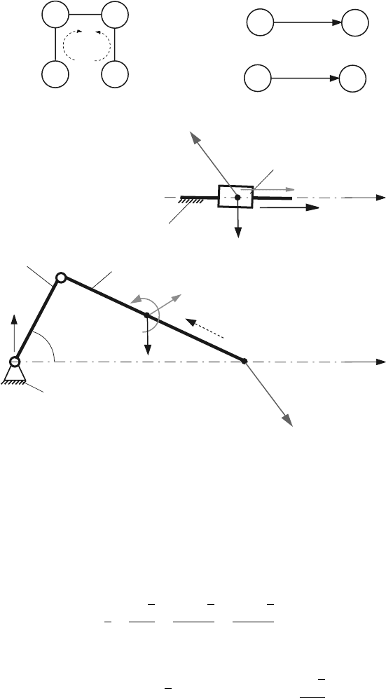
The moment M required for dynamic equilibrium is calculated from the moment
equation of for link 1 (Fig. 4.20) about the fixed point A
∑
M
(1)
A
=⇒ I
C
1
α
1
+ r
C
1
×m
1
a
C
1
= r
B
×F
21
+ G
1
+ M.
Thus, M = 151.492 N m. The joint reaction force F
01
is calculated from
∑
F
(1)
=⇒ m
1
a
C
1
= −F
12
+ G
1
+ F
01
,
4.6 Slider-Crank (R-RRT) Mechanism 139
1
A
M
B
C
1
F
21
F
21y
F
21x
G
1
Driver R
0
FBD
1
B
C
1
A
m
1
a
C
1
I
C1
α
1
NEWTON-EULER
(Kinetic Diagram)
Fig. 4.20 Newton–Euler diagram for driver link
and F
01
= −102.828ı + 116.414j N. The MATLAB program for the dyad method
and the results are given in Appendix C.3.
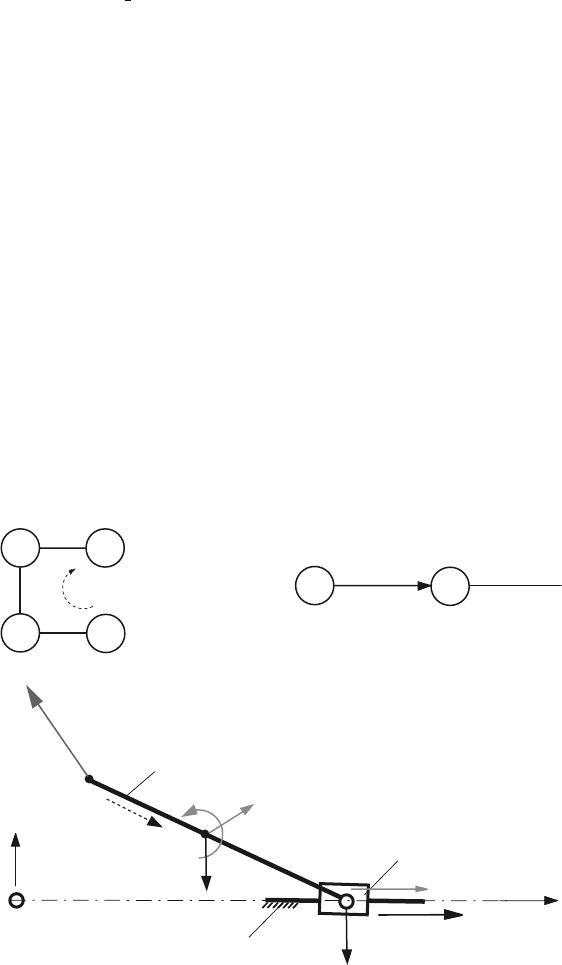
D’Alembert’s principle can be applied for the dyad method using the diagrams
shown in Fig. 4.21.
1
A
B
2
3
F
M
ext
B
C
1
C
2
C
F
21
F
12
F
in 3
G
3
F
03
G
2
F
in 2
M
in 2
F
12x
F
12y
F
21y
F
21x
F
in 1
M
in 1
G
1
Dyad RRT
Driver
R
0
Fig. 4.21 D’Alembert’s principle for the dyad method
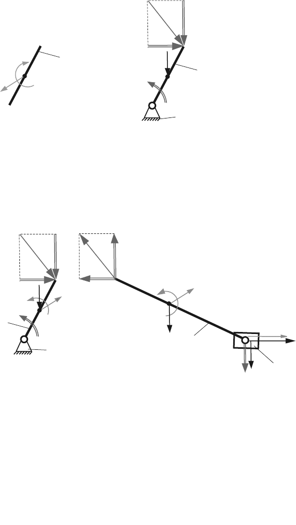
4.6.2.4 Contour Method
The diagram representing the mechanism is shown in Fig. 4.22 and has one contour,
0-1-2-3-0. The dynamic force analysis can start with any joint.
Reaction F
03
The reaction force F
03
is perpendicular to the sliding direction of joint C
T
(C
Translation
)
as shown in Fig. 4.23
F
03
= F
03y
j.
140 4 Dynamic Force Analysis
1
A
B
C
2
3
0
0
0
3
2
1
A
R
B
R
C
R
C
T
contour diagram
Fig. 4.22 Contour diagram representing the mechanism
The application point of the unknown reaction force F
03
is computed from a moment
equation about C
R
(C
Rotation
) for link 3 (path I), as shown in Fig. 4.23
∑
M
(3)
C
= r
CP
×F
03
=(r
P
−r
C
) ×F
03
= 0,
or
xF
05y
= 0 ⇒ x = 0.
The application point of the reaction force F
03
is at C (P ≡C).
The magnitude of the reaction force F
03y
is obtained from a moment equation
about B
R
for the links 3 and 2 (path I)
1
A
B
C
2
3
0
F
x
y
φ
ext
Δ
F
03
F
in 3
G
3
C
2
G
2
F
in 2
M
in 2
0
3
2
1
A
R
B
R
C
R
F
03
03
I
3
2
C
R
B
R
F
03
03
path I:
M
(3)
C
M
B
(3&2)
I
C
T
Fig. 4.23 Diagram for calculating the reaction force F
03
4.6 Slider-Crank (R-RRT) Mechanism 141
∑
M
(3&2)
B
= r
BC
×(F
03
+ F
in3
+ G
3
+ F
ext
)
+r
BC
2
×(F
in2
+ G
2
)+M
in2
= 0,
or
ıj
k
x
C
−x
B
y
C
−y
B
0
F
in3x
+ F
ext
F
03y
+ F
in3y
−m
3
g 0
+
ıj
k
x
C
2
−x
B
y
C
2
−y
B
0
F
in2x
F
in2y
−m
2
g 0
+M
in2
k = 0,
or numerically
3
2
−
5
√
2
+ 45
√
2 +
F
03y
√
2
= 0.
The reaction F
03y
is
F
03y
= −85 −
3
√
2
2
N.
The MATLAB statements for finding F
03
are:
% Joint C
T
F03=[ 0 sym(’F03y’,’real’) 0 ];
eqM32B=cross(rC-rB,F03+G3+Fin3+Fe)+...
cross(rC2-rB,Fin2+G2)+Min2;
eqM32Bz=eqM32B(3);
fprintf(’%s=0(1)\n’, char(vpa(eqM32Bz,6)))
fprintf(’Eq(1) => F03y \n’)
solF03=solve(eqM32Bz);
F03ys=eval(solF03);
F03s=[ 0, F03ys, 0 ];
fprintf(’F03 = [ %g, %g, %g ] (N)\n’, F03s)
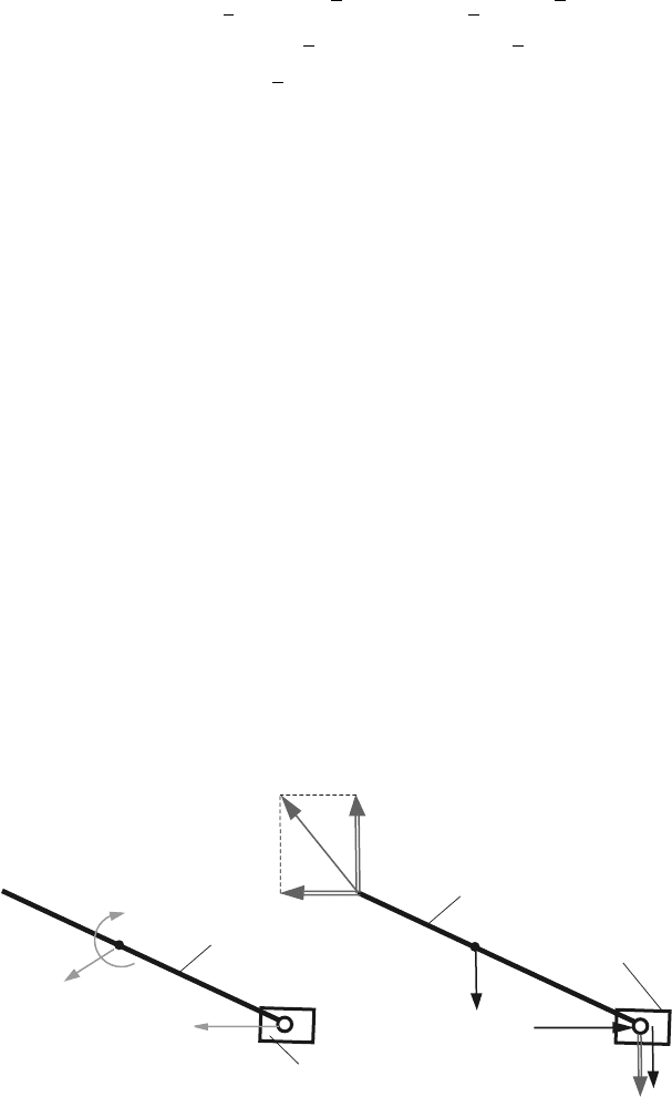
Reaction F
23
The pin joint at C
R
, between 2 and 3, is replaced with the reaction force (Fig. 4.24)
F
23
= −F
32
= F
23x
ı + F
23y
j.
For the path I, an equation for the forces projected onto the sliding direction of the
joint C
T
is written for link 3
∑
F
(3)
·ı =(F
23
+ F
in3
+ G
3
+ F
ext
) ·ı
= F
23x
+ F
in3x
+ F
ext
= F
23x
+ 100 +
√
2 = 0. (4.49)
For the path II, shown Fig. 4.24, a moment equation about B
R
is written for link 2
142 4 Dynamic Force Analysis
C
3
F
x
ext
Δ
F
in 3
G
3
1
2
3
0
C
R
A
R
C
T
B
R
F
23
23
F
32
32
I
2
1
B
R
C
T
F
32
32
path II:
M
(2)
B
F
Δ
3
0
F
23
23
path I:
(3)
II
1
A
B
2
0
x
y
φ
Δ
C
2
G
2
F
in 2
M
in 2
II
F
32
F
23
0
C
Fig. 4.24 Diagram for calculating the reaction force F
23
∑
M
(2)
B
= r
BC
×(−F
23
)+r
BC
2
×(F
in2
+ G
2
)+M
in2
= 0,
ıj
k
x
C
−x
B
y
C
−y
B
0
−F
23x
−F
23y
0
+
ıj
k
x
C
2
−x
B
y
C
2
−y
B
0
F
in2x
F
in2y
−m
2
g 0
+ M
in2
k = 0,
or numerically
1
2
−
5
√
2
2
−
F
23x
√
2
2
−
F
23y
√
2
2
= 0. (4.50)
The joint force F
23
is obtained from the system of Eqs. 4.49 and 4.50
F
23x
= −100 −
√
2 N and F
23y
= 95 +
3
√
2
2
N.
4.6 Slider-Crank (R-RRT) Mechanism 143
The MATLAB statements for finding F
23
are:
% Joint C
R
F23 = [ sym(’F23x’,’real’) sym(’F23y’,’real’) 0 ];
eqF3 = F23+Fe+G3+Fin3;
eqF3x = eqF3(1);
eqM2B = cross(rC-rB,-F23)+cross(rC2-rB,Fin2+G2)+Min2;
eqM2Bz = eqM2B(3);
fprintf(’%s=0(2)\n’, char(vpa(eqF3x,6)))
fprintf(’%s=0(3)\n’, char(vpa(eqM2Bz,6)))
fprintf(’Eqs(2)-(3) => F23x, F23y \n’)
solF23=solve(eqF3x,eqM2Bz);
F23xs=eval(solF23.F23x);
F23ys=eval(solF23.F23y);
F23s = [ F23xs, F23ys, 0 ];
fprintf(’F23 = [ %g, %g, %g ] (N)\n’, F23s)
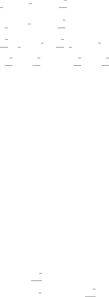
Reaction F
12
The pin joint at B
R
, between 1 and 2, is replaced with the reaction force (Fig. 4.25)
F
12
= −F
21
= F
12x
ı + F
12y
j.
For the path I, shown in Fig. 4.25, a moment equation about C
R
is written for link 2
A
B
C
2
3
F
x
y
ext
Δ
F
in 3
G
3
C
2
G
2
F
in 2
M
in 2
I
0
0
3
2
1
A
R
B
R
C
R
C
T
F
12
12
F
21
21
I
2
3
C
R
C
T
F
12
12
path I:
M
(2)
C
(2&3)
F
Δ
F
12
Fig. 4.25 Diagram for calculating the reaction force F
12
144 4 Dynamic Force Analysis
∑
M
(2)
C
= r
CB
×F
12
+ r
CC
2
×(F
in2
+ G
2
)+M
in2
= 0,
ıj
k
x
B
−x
C
y
B
−y
C
0
F
12x
F
12y
0
+
ıj
k
x
C
2
−x
C
y
C
2
−y
C
0
F
in2x
F
in2y
−m
2
g 0
+ M
in2
k = 0,
or numerically
−
1
2
+
5
√
2
2
−
F
12x
√
2
2
−
F
12y
√
2
2
= 0. (4.51)
Continuing on path I, an equation for the forces projected onto the sliding direction
of the joint C
T
is written for links 2 and 3
∑
F
(2&3)
·ı =(F
12
+ F
in2
+ G
2
+ F
in3
+ G
3
+ F
ext
) ·ı
= F
12x
+ F
in2x
+ F
in3x
+ F
ext
= F
23x
+ 100 +
√
2 +
3
√
2
2
= 0. (4.52)
The joint force F
12
is obtained from the system of Eqs. 4.52 and 4.51
F
12x
= −
1
4
(400 + 7
√
2) N and F
12y
=
5
4
(84 +
√
2) N.
The MATLAB statements for finding F
12
are:
% Joint B
R
F12 = [ sym(’F12x’,’real’) sym(’F12y’,’real’) 0 ];
eqM2C = cross(rB-rC,F12)+cross(rC2-rC,Fin2+G2)+Min2;
eqM2Cz = eqM2C(3);
eqF23 = (F12+Fin2+G2+G3+Fin3+Fe);
eqF23x = eqF23(1);
fprintf(’%s=0(4)\n’, char(vpa(eqM2Cz,6)))
fprintf(’%s=0(5)\n’, char(vpa(eqF23x,6)))
fprintf(’Eqs(4)-(5) => F12x, F12y \n’)
solF12 = solve(eqM2Cz,eqF23x);
F12xs = eval(solF12.F12x);
F12ys = eval(solF12.F12y);
F12s = [ F12xs, F12ys, 0 ];
fprintf(’F12 = [ %g, %g, %g ] (N)\n’, F12s)
Reaction F
01
and Equilibrium Moment M
The pin joint A
R
, between 0 and 1, is replaced with the unknown reaction (Fig. 4.26)
F
01
= F
01x
ı + F
01y
j.
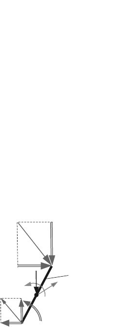
The unknown equilibrium moment is M = M k. If the path I is followed (Fig. 4.26)
for the pin joint B
R
, a moment equation is written for link 1