Dan B. Marghitu, Mechanisms and Robots Analysis with MATLAB®

Подождите немного. Документ загружается.

84 3 Velocity and Acceleration Analysis

where

¨x

d ˙x

and ¨y

d ˙y

The magnitude of the acceleration is

= a

= |a

| = |a

| =



¨x

+ ¨y

To calculate symbolically the components of the acceleration vector the following

MATLAB commands are used:

aD = diff(vD,t);

The numerical values for the acceleration of D

= D

are

¨x

= 2.5548 m/s

and ¨y

= −2.71212 m/s

and can be printed using MATLAB:

% numerical value for aD

aDn = double(subs(aD,slist,nlist));

fprintf(’aD3 = aD4 = [ %g, %g, %g ] (m/sˆ2) \n’, aDn)

fprintf(’|aD3| = |aD4| = %g (m/sˆ2) \n’, norm(aDn))

The angle φ

(t)=φ

(t) is determined as a function of time t from the equation of

the slope of the line BC:

tanφ

(t)=tan φ

(t)=

(t) −y

(t) −x

The MATLAB function atan(z) gives the arc tangent of the number z and the

angle φ

is calculated symbolically:

phi2 = atan((yB-yC)/(xB-xC));

The numerical value is given by:

phi2n = subs(phi2,’phi(t)’,pi/6);

The numerical solution is printed using MATLAB:

fprintf(’phi2 = phi3 = %g (degrees) \n’, phi2n

180/pi)

The angular velocity ω

(t)=ω

(t) is the derivative with respect to time of the angle

(t)

dφ

(t)

3.9 Derivative Method 85

Symbolically, the angular velocity ω

= ω

is calculated using MATLAB:

% omega2 in terms of phi(t) and diff(’phi(t)’,t)

dphi2 = diff(phi2,t);

and is the numerical value is printed using the MATLAB statements:

dphi2nn = subs(dphi2,diff(’phi(t)’,t),omega);

dphi2n = subs(dphi2nn,’phi(t)’,pi/6);

fprintf(’omega2 = omega3 = %g (rad/s) \n’, dphi2n)

The angular acceleration α

(t)=α

(t) is the derivative with respect to time of the

angular velocity ω

(t):

(t)=

dω

(t)

Symbolically, using MATLAB, the angular acceleration α

is:

ddphi2 = diff(dphi2,t);

The numerical solution is printed using MATLAB:

ddphi2n = double(subs(ddphi2,slist,nlist));

fprintf(’alpha2 = alpha3 = %g (rad/s ˆ2) \n’, ddphi2n)

The numerical values of the angles, angular velocities, and angular accelerations for

the links 2 and 3 are:

= φ

= −10.8934 rad, ω

= ω

= 4.48799 rad/s, α

= α

= 14.5363 rad/s

The angle φ

(t)=φ

(t) is determined as a function of time t from the following

equation:

tanφ

(t)=tan φ

(t)=

(t) −y

(t) −x

and symbolically using MATLAB:

ddphi4 = diff(dphi4,t);

The angular velocity ω

(t)=ω

(t) is the derivative with respect to time of the angle

(t)

dφ

(t)

86 3 Velocity and Acceleration Analysis

To calculate symbolically the angular velocity ω

using MATLAB, the following

command is used:

dphi4 = diff(phi4,t);

The angular acceleration α

(t)=α

(t) is the derivative with respect to time of the

angular velocity ω

(t):

(t)=

dω

(t)

and it is calculated symbolically with MATLAB:

ddphi4 = diff(dphi4,t);

The numerical values of the angles, angular velocities, and angular accelerations for

the links 5 and 4 are:

= φ

= 138.933 rad, ω

= ω

= 2.97887 rad/s, α

= α

= 12.1939 rad/s

The numerical solutions printed with MATLAB are:

dphi4n = double(subs(dphi4,slist,nlist));

fprintf(’omega4 = omega5 = %g (rad/s) \n’, dphi4n)

ddphi4n = double(subs(ddphi4,slist,nlist));

fprintf(’alpha4 = alpha5 = %g (rad/sˆ2) \n’, ddphi4n)

The MATLAB program for velocity and acceleration analysis and the results are

given in Appendix B.5.

Exercise: Inverted Slider-Crank Mechanism

The mechanism considered in Sect. 3.7 (shown in Fig. 3.6) will be analyzed using

the derivative method. The dimensions of the links are AC=0.15 m and BC=0.2 m.

The driver link 1 rotates with a constant speed of n = n

= 30 rpm.

Find the velocities and the accelerations of the mechanism when the angle of the

driver link 1 with the horizontal axis is φ = φ

= 60

◦

Solution

A Cartesian reference frame with the origin at A is selected. The coordinates of joint

A are x

= y

= 0. The coordinates of the joint C are x

= AC = 0.15 m and y

= 0.

The position of joint B is calculated from the equations

tanφ (t)=

(t)

and [x

(t) −x

]

+[y

(t) −y

]

= BC

3.9 Derivative Method 87

(t) sin φ (t)=y

(t) cos φ (t),

(t) −x

]

+[y

(t) −y

]

= BC

. (3.82)

The coordinates of joint B are x

= 0.113535 m and y

= 0.196648 m. The MAT-

LAB statements for the positions are:

AC=0.15;BC=0.20;xA=0;yA=0;

xC=AC;yC=0;

n = 30 ; omega = n

pi/30;

t = sym(’t’,’real’) ;

phi = sym(’phi(t)’) ;

xB = sym(’xB(t)’) ;

yB = sym(’yB(t)’) ;

eqB1 = xB

sin(phi) - yB

cos(phi) ;

eqB2=(xB-xC)ˆ2+(yB-yC)ˆ2-BCˆ2 ;

sp = {’phi(t)’,’xB(t)’,’yB(t)’} ;

np = {pi/3,’xBn’,’yBn’} ;

eqB1p = subs(eqB1,sp,np) ;

eqB2p = subs(eqB2,sp,np) ;

solBp = solve(eqB1p, eqB2p) ;

xBpositions = eval(solBp.xBn) ;

yBpositions = eval(solBp.yBn) ;

xB1 = xBpositions(1); xB2 = xBpositions(2) ;

yB1 = yBpositions(1); yB2 = yBpositions(2) ;

if yB1 > 0 xBp = xB1; yBp = yB1;

else xBp = xB2; yBp = yB2; end

rB = [xBp yBp 0] ;

fp = {pi/3,xBp,yBp} ;

The linear velocity of point B onlink3or2is

= v

= ˙x

ı + ˙y

where

˙x

and ˙y

The velocity analysis is carried out by differentiating Eq. 3.82:

˙x

sinφ + x

φ cosφ = ˙y

cosφ −y

φ sinφ,

˙x

−x

)+ ˙y

−y

)=0,

88 3 Velocity and Acceleration Analysis

˙x

sinφ + x

ω cos φ = ˙y

cosφ −y

ω sin φ ,

˙x

−x

)+ ˙y

−y

)=0. (3.83)

The magnitude of the angular velocity of the driver link 1 is

ω = ω

φ =

π n

π (30 rpm)

= 3.141 rad/s.

The link 2 and the driver link 1 have the same angular velocity

= ω

. For the

given numerical data Eq. 3.83 becomes

˙x

sin60

◦

+ 0.113535(3.141) cos 60

◦

= ˙y

cos60

◦

−0.196648(3.141) sin 60

◦

˙x

(0.113535 −0.15)+ ˙y

(0.196648 −0)=0. (3.84)

The solution of Eq. 3.84 gives

˙x

= −0.922477 m/s and ˙y

= −0.17106 m/s.

The velocity of B is

= v

= −0.922477ı −0.17106 j m/s,

| = |v

| =



(−0.922477)

+(−0.17106)

= 0.938203 m/s.

The MATLAB statements for the velocity of B

= B

are:

deqB1 = diff(eqB1,t) ;

deqB2 = diff(eqB2,t) ;

sv = ...

{diff(’phi(t)’,t),diff(’xB(t)’,t),diff(’yB(t)’,t)};

nv = {omega,’vxB’,’vyB’} ;

deqB1p=subs(deqB1,sv,nv) ;

deqB1n=subs(deqB1p,sp,fp) ;

deqB2p=subs(deqB2,sv,nv) ;

deqB2n=subs(deqB2p,sp,fp) ;

solvB = solve(deqB1n, deqB2n) ;

vBx = eval(solvB.vxB) ;

vBy = eval(solvB.vyB) ;

fv = {omega,vBx,vBy} ;

The acceleration analysis is obtained using the derivative of the velocities given by

Eq. 3.83:

3.9 Derivative Method 89

¨x

sinφ + ˙x

ω cos φ + ˙x

ω cos φ −x

sinφ

= ¨y

cosφ − ˙y

ω sin φ − ˙y

ω sin φ + y

cosφ ,

¨x

−x

)+ ˙x

+ ¨y

−y

)+ ˙y

= 0. (3.85)

The magnitude of the angular acceleration of the driver link 1 is

α =

ω =

φ = 0.

Numerically, Eq. 3.85 gives

¨x

sin60

◦

+ 2(−0.922477)(3.141) cos60

◦

−0.113535(3.141)

sin60

◦

= ¨y

cos45

◦

−2(−0.17106)(3.141) sin60

◦

+ 0.196648(3.141)

cos60

◦

¨x

(0.113535 −0.15) ¨y

(0.196648 −0)

+(−0.922477)

+(−0.17106)

= 0. (3.86)

The solution of Eq. 3.86 is

¨x

= 2.0571 m/s

and ¨y

= −4.0947 m/s

The acceleration of B onlink3or2is

= a

= ¨x

ı + ¨y

j = 2.0571ı −4.0947 j m/s

| = |a

| =



(2.0571)

+(−4.0947)

= 4.58238 m/s

The MATLAB statements for the acceleration of B

= B

are:

ddeqB1 = diff(deqB1,t) ;

ddeqB2 = diff(deqB2,t) ;

sa={diff(’phi(t)’,t,2),diff(’xB(t)’,t,2),...

diff(’yB(t)’,t,2)};

na={0,’axB’,’ayB’} ;

ddeqB1p=subs(ddeqB1,sa,na) ;

ddeqB1n=subs(ddeqB1p,sv,fv) ;

ddeqB1f=subs(ddeqB1n,sp,fp) ;

ddeqB2p=subs(ddeqB2,sa,na) ;

ddeqB2n=subs(ddeqB2p,sv,fv) ;

ddeqB2f=subs(ddeqB2n,sp,fp) ;

solaB = solve(ddeqB1f, ddeqB2f) ;

aBx = eval(solaB.axB) ;

90 3 Velocity and Acceleration Analysis

aBy = eval(solaB.ayB) ;

fa = {0,aBx,aBy};

The slope of the link 3 (the points B and C are on the straight line BC)is

tanφ

(t)=

(t) −y

(t) −x

] sinφ

(t)=[y

(t) −y

] cosφ

(t). (3.87)

The angle φ

is computed as follows:

= arctan

−y

−x

= arctan

0.196648 −0

0.113535 −0.15

= −79.4946

◦

The derivative of Eq. 3.87 yields

˙x

sinφ

+(x

−x

)

cosφ

= ˙y

cosφ

−(y

−y

)

sinφ

˙x

sinφ

+(x

−x

)ω

cosφ

= ˙y

cosφ

−(y

−y

)ω

sinφ

, (3.88)

where ω

Numerically, Eq. 3.88 gives

−0.922477 sin(−79.4946

◦

)+(0.113535 −0.15) ω

cos(−79.4946

◦

)

= −0.17106 cos(−79.4946

◦

) −(0.196648 −0)ω

sin(−79.4946

◦

with the solution ω

= 4.69102 rad/s.

The angular velocity of link 3 is

= ω

k = 4.69102k rad/s.

The MATLAB statements for the angular velocity of link 3 are:

phi3 = atan((yB-yC)/(xB-xC)) ;

phi3n = subs(phi3,sp,fp) ;

dphi3 = diff(phi3,t) ;

dphi3nn = subs(dphi3,sv,fv) ;

dphi3n = subs(dphi3nn,sp,fp) ;

fprintf(’omega3 = %g (rad/s) \n’, double(dphi3n))

The angular acceleration of link 3, α

, is obtained using the derivative of

Eq. 3.88:

3.9 Derivative Method 91

¨x

sinφ

+ ˙x

cosφ

+ ˙x

cosφ

+(x

−x

)

cosφ

−(x

−x

)ω

sinφ

= ¨y

cosφ

− ˙y

sinφ

−˙y

sinφ

−(y

−y

)

sinφ

−(y

−y

)ω

cosφ

¨x

sinφ

+ 2˙x

cosφ

+(x

−x

)α

cosφ

−(x

−x

)ω

sinφ

= ¨y

cosφ

−2˙y

sinφ

−(y

−y

)α

sinφ

−(y

−y

)ω

cosφ

Numerically, the previous equation becomes

2.0571 sin(−79.4946

◦

)+2(−0.922477)(4.69102) cos(−79.4946

◦

)

+(0.113535 −0.15)α

cos(−79.4946

◦

)

−(0.113535 −0.15)(4.69102)

sin(−79.4946

◦

)

= −4.0947 cos(−79.4946

◦

) −2(−0.17106)(4.69102) sin(−79.4946

◦

)

−(0.196648 −0)α

sin(−79.4946

◦

)

−(0.196648 −0)(4.69102)

cos(−79.4946

◦

with the solution α

= −6.38024 rad/s

. The angular acceleration of link 3 is

= α

k = −6.38024k rad/s

The MATLAB statements for the angular acceleration of link 3 are:

ddphi3 = diff(dphi3,t) ;

ddphi3nnn = subs(ddphi3,sa,fa) ;

ddphi3nn = subs(ddphi3nnn,sv,fv) ;

ddphi3n = subs(ddphi3nn,sp,fp) ;

fprintf(’alpha3 = %g (rad/sˆ2 ) \n’, double(ddphi3n))

The MATLAB program for velocity and acceleration analysis and the results using

the derivative method are given in Appendix B.6.

Exercise: R-RTR Mechanism

The R-RTR mechanism shown in Fig. 3.9 has the dimensions: AB = 0.1m,AC =

0.1 m, and CD = 0.3 m. The constant angular speed of the driver link 1 is ω = ω

π rad/s.

Find the velocities and the accelerations of the mechanism using the derivative

method when the angle of the driver link 1 with the horizontal axis is φ = φ

π/4 = 45

◦

Solution

The origin of the ﬁxed reference frame is at C ≡ 0. The position of the ﬁxed joint A

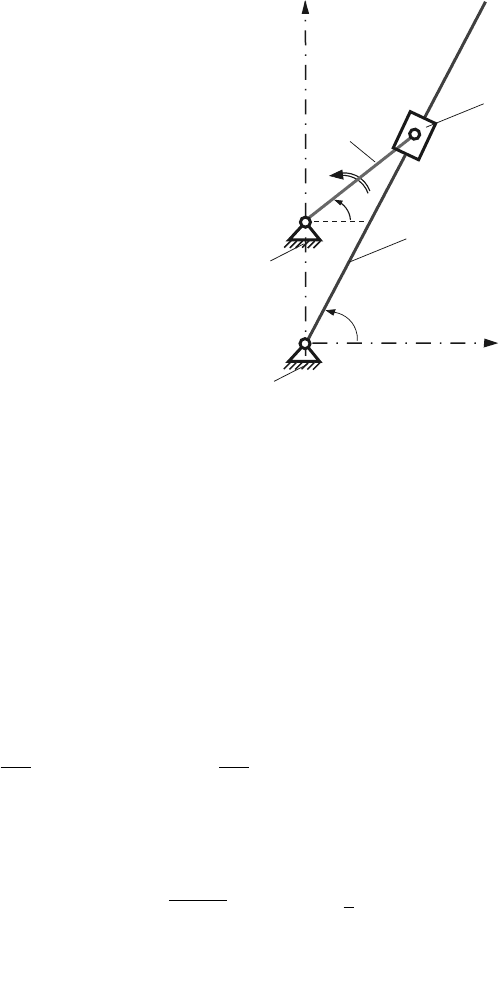
92 3 Velocity and Acceleration Analysis

Fig. 3.9 R-RTR mechanism

is x

= 0 and y

= AC = 0.1 m. The position of joint B is

(t)=x

+ AB cosφ (t), y

(t)=y

+ AB sinφ (t),

and for φ = 45

◦

, the position is

= 0 + 0.1 cos45

◦

= 0.07071 m, y

= 0.1 + 0.1 sin45

◦

= 0.17071 m.

The linear velocity vector of B

= B

= v

= ˙x

ı + ˙y

where

˙x

= −AB

φ sinφ, ˙y

= AB

φ cosφ.

With φ = 45

◦

and

φ = ω = π = 3.141 rad/s:

˙x

= −0.1π sin 45

◦

= −0.222144 m/s,

˙y

= 0.1π cos 45

◦

= −0.222144 m/s,

= v

= |v

| = |v

| =



˙x

+ ˙y

= 0.222144

√

2 m/s.

The linear acceleration vector of B

= B

= a

= ¨x

ı + ¨y

where

3.9 Derivative Method 93

¨x

d ˙x

= −AB

cosφ −AB

φ sinφ,

¨y

d ˙y

= −AB

sinφ + AB

φ cosφ.

The angular acceleration of link 1 is

φ =

ω = α = 0. The numerical values for the

acceleration of B are

¨x

= −0.1π

cos45

◦

−0 = −0.697886 m/s

¨y

= −0.1π

sin45

◦

+ 0 = −0.697886 m/s

= a

= |a

| = |a

| =



¨x

+ ¨y

= 0.697886

√

2 m/s

The MATLAB statements for the velocity and acceleration of B

= B

are:

AB = 0.1; AC = 0.1; CD = 0.3; % (m)

phi1 = pi/4; omega = pi; alpha = 0;

xC=0;yC=0;

xA=0;yA=AC;

t = sym(’t’,’real’);

xB1=xA+AB

cos(sym(’phi(t)’));

yB1=yA+AB

sin(sym(’phi(t)’));

rB = [ xB1 yB1 0 ]; %symbolic function of phi(t)

xBn = subs(xB1,’phi(t)’,pi/4); % xB for phi(t)=pi/4

yBn = subs(yB1,’phi(t)’,pi/4); % yB for phi(t)=pi/4

rBn = subs(rB,’phi(t)’,pi/4); % rB for phi(t)=pi/4

fprintf(’rB = [ %g, %g, %g ] (m)\n’, rBn)

vB = diff(rB,t); %differentiates rB with respect to t

%list for symbolical variables phi’’,phi’,phi

slist={diff(’phi(t)’,t,2),diff(’phi(t)’,t),’phi(t)’};

%list for numerical values of phi’’(t),phi’(t),phi(t)

nlist={alpha,omega,phi1}; %numerical values for slist

vBn = double(subs(vB,slist,nlist));

fprintf(’vB1 = vB2 = [ %g, %g, %g ] (m/s)\n’, vBn)

fprintf(’|vB1| = |vB2| = %g (m/s)\n’, norm(vBn))

%acceleration of B1=B2

aB = diff(vB,t); %differentiates vB with respect to t

aBn = double(subs(aB,slist,nlist));

fprintf(’aB1 = aB2 = [ %g, %g, %g ] (m/sˆ2)\n’, aBn)

fprintf(’|aB1| = |aB2| = %g (m/sˆ2)\n’, norm(aBn))

The points B and C are located on the same straight line BCD:

(t) −y

−[x

(t) −x

] tanφ

(t)=0. (3.89)