Cox R. Partial Differential Equations

Подождите немного. Документ загружается.

In one dimension, recall that the second derivative measures concavity. Suppose y = f(x);

if f''(x) is positive, y is concave up, and if f''(x) is negative, y is concave down. The

Laplacian may be thought of as a generalization of the concavity concept to multivariate

functions.

This idea is demonstrated at the right, in one dimension: u(x) = x

− x. To the left of x = 0,

the Laplacian (simply the second derivative here) is negative, and the graph is concave

down. At x = 0, the curve inflects and the Laplacian is 0. To the right of x = 0, the

Laplacian is positive and the graph is concave up.

Concavity may or may not do it for you. Thankfully, there's another very important view

of the Laplacian, with deep implications for any equation it shows itself in: the Laplacian

compares the value of u at some point in space to the average of the values of u in the

neighborhood of the same point. The three cases are:

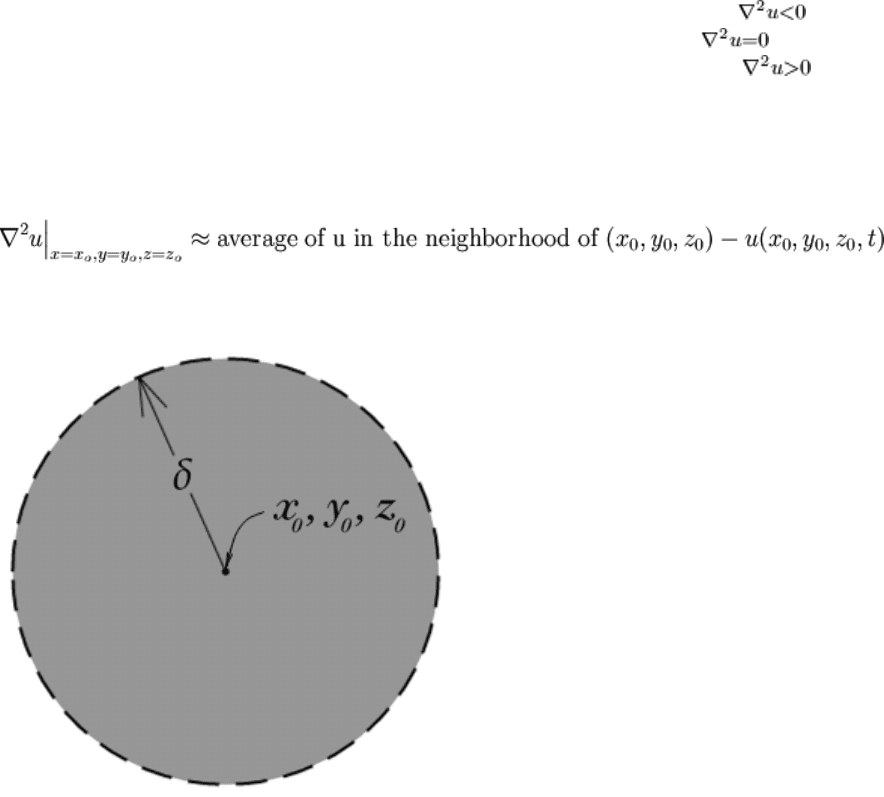
 If u is greater at some point then the average of its neighbors, .

 If u is at some point equal to the average of its neighbors, .

 If u is smaller at some point then the average of its neighbors, .

So the laplacian may be thought of as, at some point (x

The neighborhood of (x

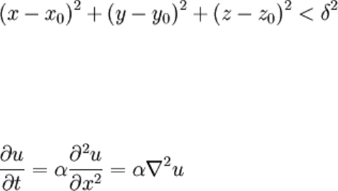
The neighborhood of some point is defined as the open set that lies within some

Euclidean distance δ from the point. Referring to the picture at right (a 3D example), the

neighborhood of the point (x

) is the shaded region which satisfies:

Note that our one dimensional transient diffusion equation involves the Laplacian:

With this mentality, let's examine the behavior of this very important PDE. On the left is

the time derivative and on the right is the Laplacian. This equation is saying that:

The rate of change of u at some point is proportional to the difference

between the average value of u around that point and the value of u at that

point.

For example, if there's at some position a "hot spot" where u is on average greater then its

neighbors, the Laplacian will be negative and thus the time derivative will be negative,

this will cause u to decrease at that position, "cooling" it down. This is illustrated below.

The arrows reflect upon the magnitude of the Laplacian and, by grace of the time

derivative, the direction the curve will move.

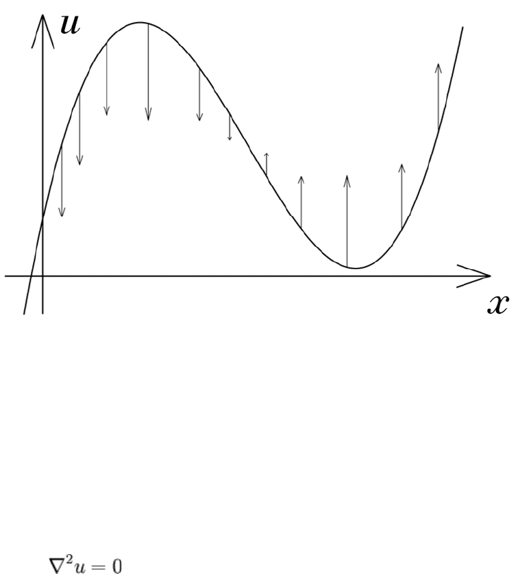
Visualization of transient diffusion.

It's worth noting that in 3D, this equation fully describes the flow of heat in a

homogeneous solid that's not generating it's own heat (like too much electricity through a

narrow wire would).

Laplace's Equation

Laplace's equation describes a steady state condition, and this is what it looks like:

Solutions of this equation are called harmonic functions. Some things to note:

 Time is absent. This equation describes a steady state condition.

 The absence of time implies the absence of an IC, so we'll be dealing with

BVPs rather then IBVPs.

 In one dimension, this is the ODE of a straight line passing through the

boundaries at their specified values.

 All functions that satisfy this equation in some domain are analytic

(informally, an analytic function is equal to its Taylor expansion) in that

domain.

 Despite appearances, solutions of Laplace's equation are generally not

minimal surfaces.

 Laplace's equation is linear.

Laplace's equation is separable in the Cartesian (and almost any other) coordinate system.

So, we shouldn't have too much problem solving it if the BCs involved aren't too

convoluted.

Laplace's Equation on a Square: Cartesian Coordinates

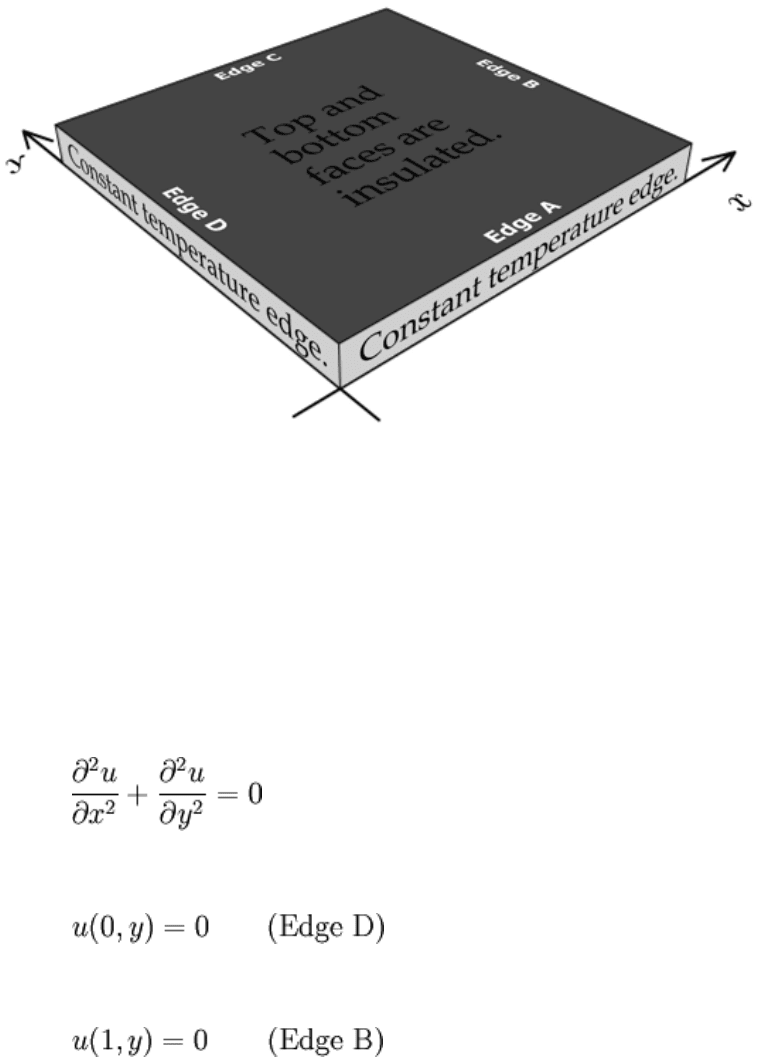
Steady state conditions on a square.

Imagine a 1 x 1 square plate that's insulated top and bottom and has constant

temperatures applied at its uninsulated edges, visualized to the right. Heat is flowing in

and out of this thing steadily through the edges only, and since it's "thin" and "insulated",

the temperature may be given as u(x,y). This is the first time we venture into two spatial

coordinates, note the absence of time.

Let's make up a BVP, referring to the picture:

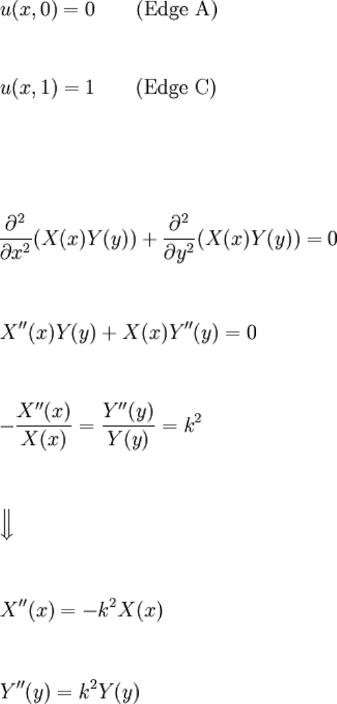
So we have one nonhomogeneous BC. Assume that u(x,y) = X(x)Y(y):

As with before, calling the separation constant k

in favor of just k (or something)

happens to make the problem easier to solve. Note that the negative sign was kept for the

X(x) equation: again, these choices happen to make things simpler. Solving each equation

and combining them back into u(x,y):

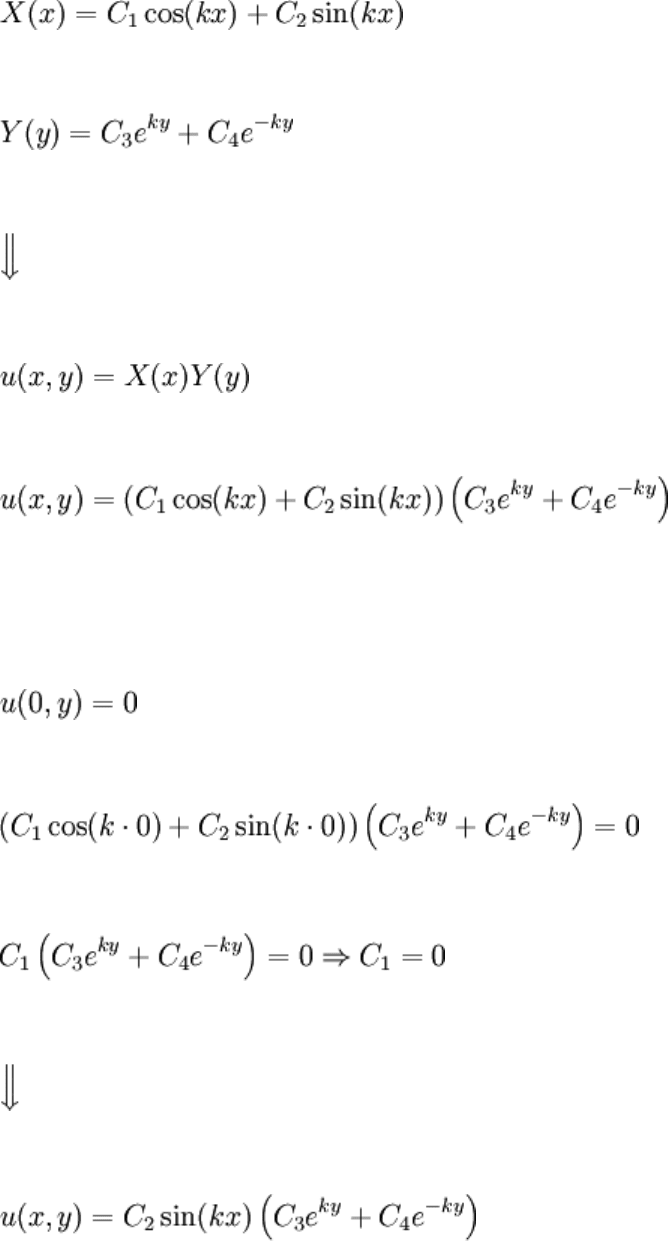
At edge D:

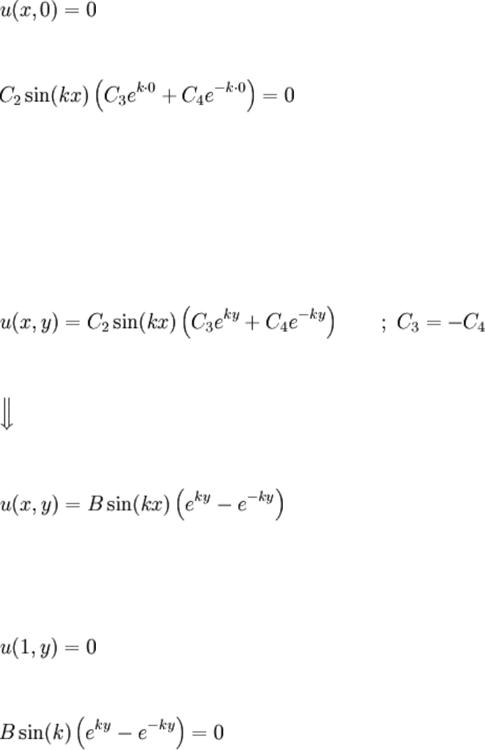
Note that the constants can be merged, but we won't do it so that a point can be made in a

moment. At edge A:

Taking C

as 0 would satisfy this particular BC, however this would yield a plane

solution of u(x,y) = 0, which can't satisfy the temperature at edge C. This is why the

constants weren't merged a few steps ago, to make it obvious that C

may not be 0. So,

we instead take C

= − C

to satisfy the above, and then combine the three constants into

one, call it B:

Now look at edge B:

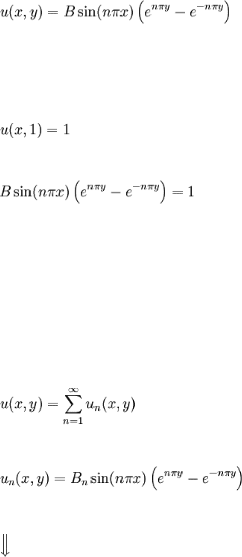
It should go without saying by now that B can't be zero, since this would yield u(x,y) = 0

which couldn't satisfy the nonzero BC. Instead, we can take k = nπ:

As of now, this solution will satisfy 3 of the 4 BCs. All that is left is edge C, the

nonhomogeneous BC.

Neither B nor n can be contorted to fit this BC.

Since Laplace's equation is linear, a linear combination of solutions to the PDE is also a

solution to the PDE. Another thing to note: since the BCs (so far) are homogeneous, we

can add the solutions without worrying about nonzero boundaries adding up.

Though u(x,y) as shown above will not solve this problem, we can try summing (based on

n) solutions to form a linear combination which might solve the BVP as a whole:

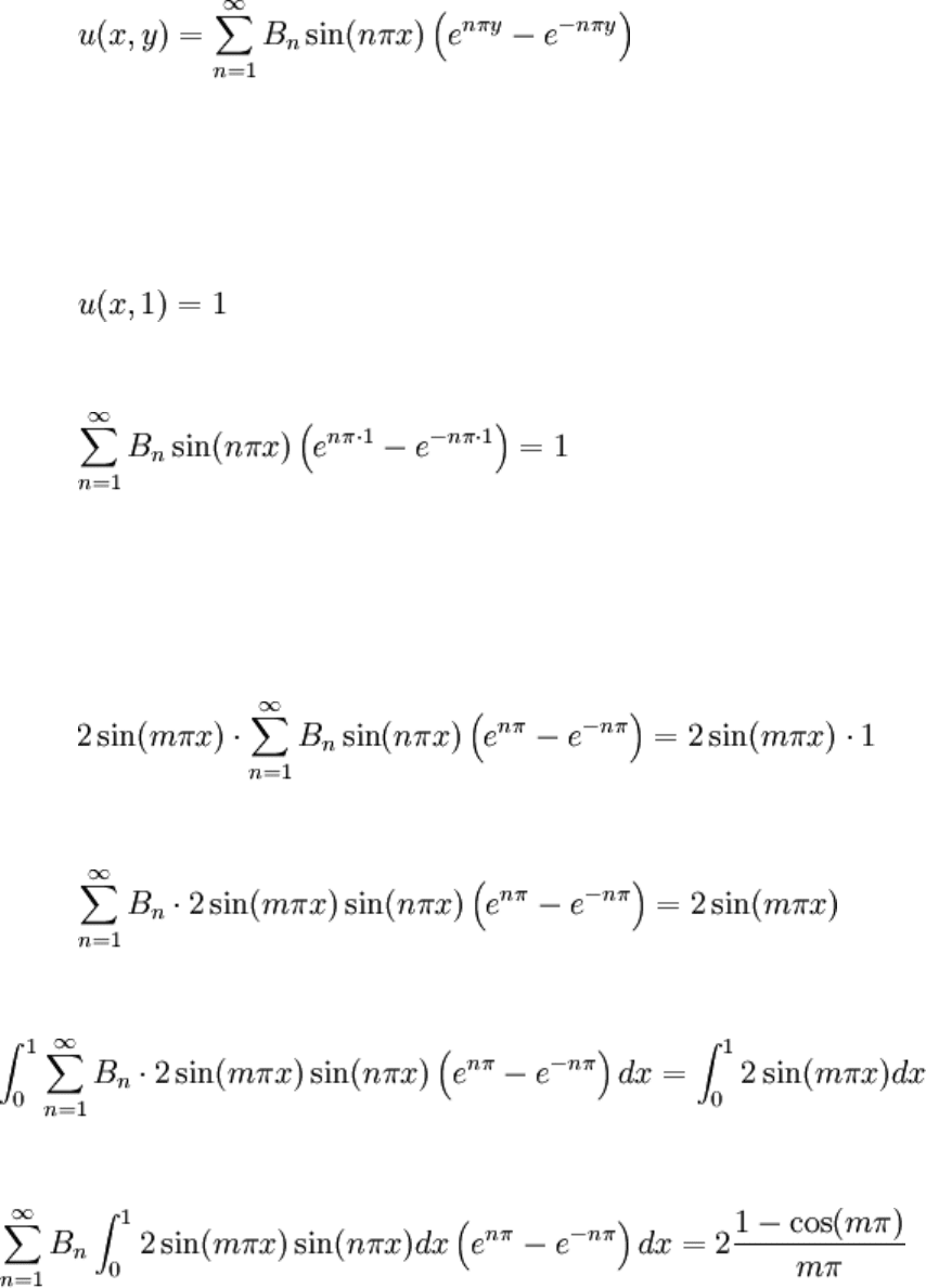
Assuming this form is correct (review Parallel Plate Flow: Realistic IC for motivation),

let's again try applying the last BC:

It looks like it needs Fourier series methodology. Finding B

via orthogonality should

solve this problem:

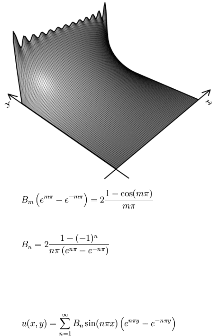
25 term partial sum of the series solution.

m was changed to n in the last step. Also, for integer n, cos(nπ) = ( − 1)

. Note that a

Fourier sine expansion has been done. The solution to the BVP can finally be assembled: