Coburn J.W., Herdlick J.D. College Algebra: Graphs and Models
Подождите немного. Документ загружается.


4. To help “round-out” the graph we evaluate the midinterval point using
the remainder theorem or the factored form of g(x), which shows that
is also a point on the graph.
use as a “divisor”
The final result is the graph shown.
Now try Exercises 57 through 72
䊳
2
|
10 9 4 12
2 4 10 28
12 514
|
16
2
12, 162
x 2
420 CHAPTER 4 Polynomial and Rational Functions 4–40
College Algebra Graphs & Models—
CAUTION
䊳
Sometimes using a midinterval point to help draw a graph will give the illusion that a
maximum or minimum value has been located. This is rarely the case, as demonstrated
in the figure in Example 8, where the maximum value in Quadrant II is actually closer to
12.22, 16.952.
EXAMPLE 9
䊳
Using the Guidelines to Sketch a Polynomial Graph
Sketch the graph of
Solution
䊳
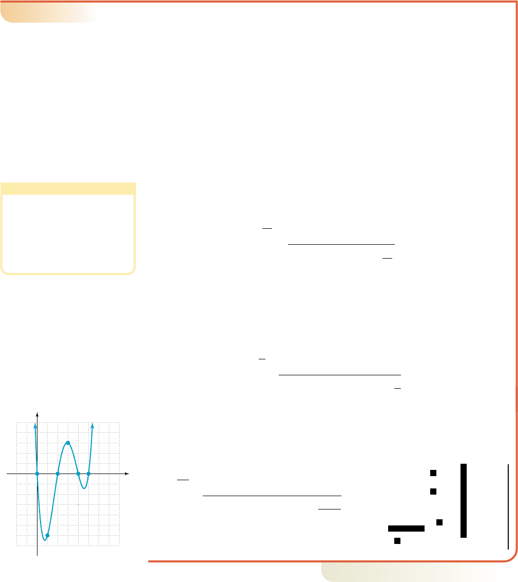
1. End-behavior: The function has degree 7 (odd) so the ends will point in
opposite directions. The leading coefficient is positive and the end-behavior
will be down on the left and up on the right.
2. y-intercept: Since the y-intercept is (0, 0).
3. Zeroes: Testing 1 and shows neither are zeroes but (1, 4) and
are points on the graph. Factoring out produces
and we see that is a zero of multiplicity 3. We next use
synthetic division with on the fourth-degree polynomial:
use 2 as a “divisor”
This shows is a zero and is a
factor. At this stage, it appears the quotient
can be factored by grouping. From
we
obtain
after factoring and
as the completely factored form. We find
that is a zero of multiplicity 2, and
the remaining two zeroes are complex.
4. Using this information produces the graph shown in the figure.
Now try Exercises 73 through 76
䊳
For practice with these ideas using a graphing calculator, see Exercises 77 through 80.
Similar to our work in previous sections, Exercises 81 and 82 ask you to reconstruct
the complete equation of a polynomial from its given graph.
x 2
h1x2 x
3
1x 22
2
1x
2
32
h1x2 x
3
1x 221x
2
321x 22
h1x2 x
3
1x 221x
3
2x
2
3x 62,
x 2x 2
2
|
1 4712 12
2 4612
1 236|0
x 2
x 012x 122,
h1x2 x
3
1x
4
4x
3
7x
2
x
3
11, 3621
h102 0,
h1x2 x
7
4x
6
7x
5
12x
4
12x
3
.
33
10
10
Down on
left
Up on
right
(0, 0)
(2, 0)
(1, 4)
h(x)
x
y
D. You’ve just seen how
we can graph polynomial
functions in standard form
cob19545_ch04_411-429.qxd 8/19/10 11:12 PM Page 420
4–41 Section 4.3 Graphing Polynomial Functions 421
College Algebra Graphs & Models—
E. Applications of Polynomials and Polynomial Modeling
EXAMPLE 10
䊳
Modeling the Value of an Investment
In the year 2000, Marc and his wife Maria decided to invest some money in precious
metals. As expected, the value of the investment fluctuated over the years, sometimes
being worth more than they paid, other times less. Suppose that through 2010, the gain
or loss on the investment was modeled by where v(t)
represents the gain or loss (in hundreds of dollars) in year t
a. Use the rational zeroes theorem to find the years when their gain/loss was zero.
b. Sketch the graph of the function.
c. In what years was the investment worth less than they paid?
d. What was their gain or loss in 2010?
Solution
䊳
a. Writing the function as we note shows
no gain or loss on purchase, and attempt to find the remaining zeroes. Testing
for 1 and shows neither is a zero, but and are points on
the graph of v. Next we try with the factor theorem and the cubic
polynomial.
We find that 2 is a zero and write then factor to
obtain Since for 2, 4, and 5, they
“broke even” in years 2000, 2002, 2004, and 2005.
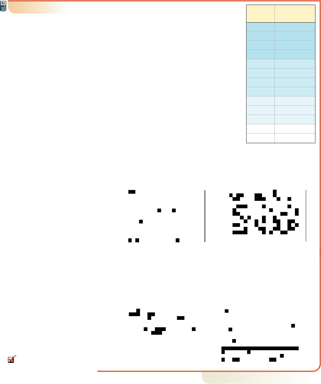
b. With even degree and a positive leading coefficient, the end-behavior is up/up.
All zeroes have multiplicity 1. As an additional midinterval point we find
The graph is shown in Figure 4.26.
c. The investment was worth less than what they paid (outputs are negative) from
2000 to 2002 and 2004 to 2005.
d. In 2010, they were “sitting pretty,” as their
investment had gained $2,400.
These values can also be calculated or
confirmed using a graphing calculator.
See Figure 4.27.
Now try Exercises 85 through 88
䊳
As with linear and quadratic regression models, applications of other polynomial
models begins with a scatterplot and a decision as to which form of regression might
be appropriate. This can depend on a number of factors, such as any end-behavior that is
10
|
1 11 38 40 0
10 10 280 2400
1 1 28 240
|
2400
3
|
1 11 38 40 0
3 24 42 6
1 814 2
|
6
v132 6:
t 0,v1t2 0v1t2 t1t 221t 421t 52.
v1t2 t1t 221t
2
9t 202,
2
|
1 11 38 40
2 18 40
1 920
|
0
t 2
11, 90211, 1221
t 0v1t2 t1t
3
11t
2
38t 402,
1t 0 S 20002.
v1t2 t
4
11t
3
38t
2
40t,
WORTHY OF NOTE
Due to the context, the domain of
v(t) in Example 10 actually begins
at which we could designate
with a point at (0, 0). In addition,
note there are three sign changes in
the terms of v(t), indicating there
will be 3 or 1 positive roots (we
found 3).
t 0,
5
10
10
(1, 12)
(3, 6)
x
y
Figure 4.26
Figure 4.27
cob19545_ch04_411-429.qxd 8/19/10 11:12 PM Page 421
422 CHAPTER 4 Polynomial and Rational Functions 4–42
College Algebra Graphs & Models—
evident, the number of apparent turning points, any anticipated behavior, and so on.
However, due to the end-behavior of polynomial models, great care must be exercised
when these models are used to make projections beyond the limits of the given data.
EXAMPLE 11
䊳
The Earth’s atmosphere consists of several layers that
are defined in terms of altitude and the characteristics
of the air in each layer. In order, these are the
Troposphere (0–12 km), Stratosphere (12–50 km),
Mesosphere (50–80 km), and Thermosphere
(80–100 km). Due to their chemical and physical
characteristics, the air temperature within each layer
and from layer to layer varies a great deal. The data
in the table gives the temperature in at an altitude
of h kilometers (km). Use the data to:
a. Draw a scatterplot and decide on an appropriate
form of regression, then find the regression
equation.
b. Use the regression equation to find the
temperature at altitudes of 32.6 km and 63.6 km.
c. As the space shuttle rockets into orbit, a
temperature reading of is taken. What are
the possible altitudes for the shuttle at this point?
Solution
䊳
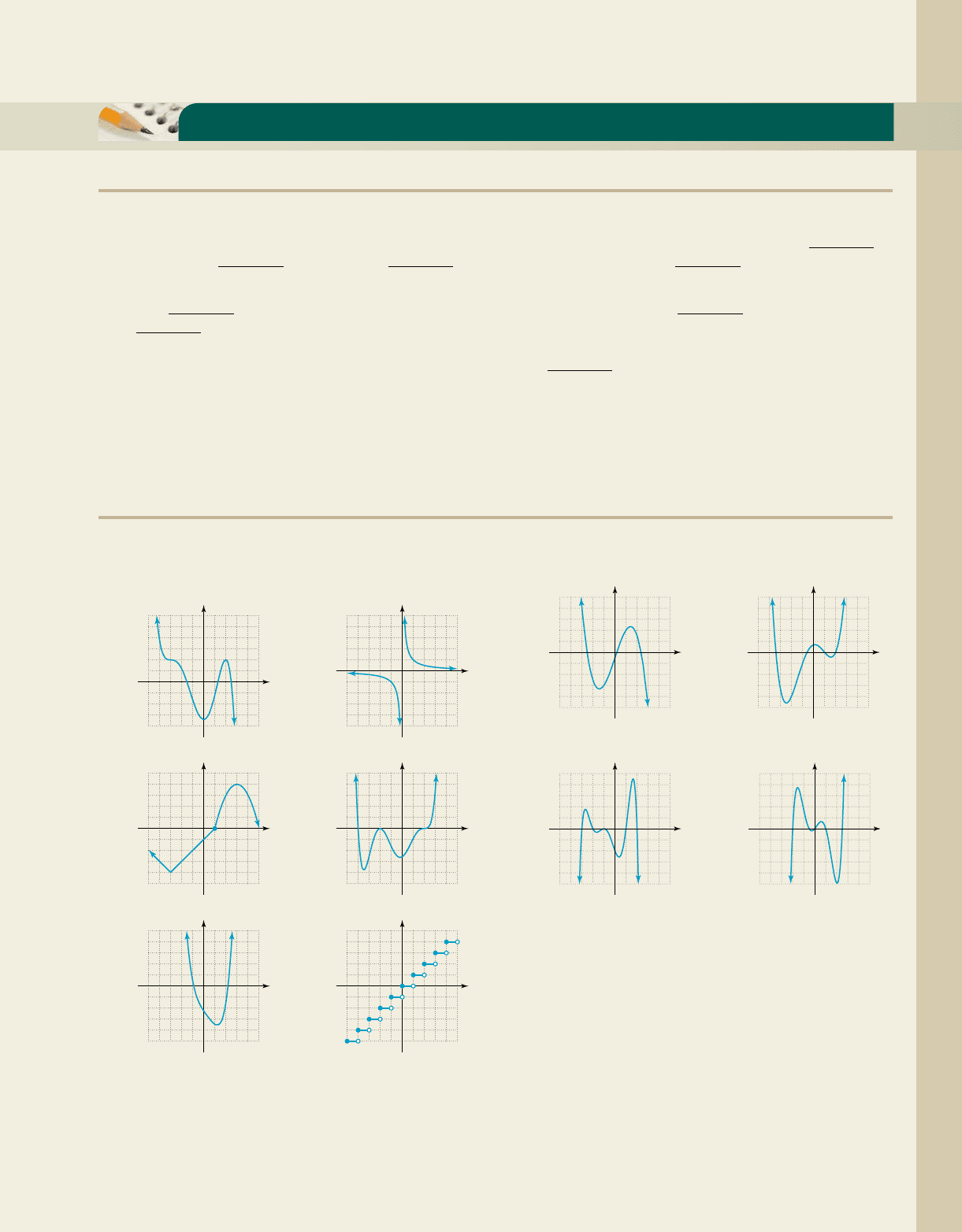
a. The scatterplot is shown in Figure 4.28. Using the characteristics exhibited
(end-behavior, three turning points), it appears a quartic regression (degree 4)
is appropriate and the equation is shown in Figure 4.29.
b. At altitudes of 32.6 km and 63.6 km, the temperature is very near
(Figure 4.30).
c. Setting , we note the line intersects the graph in two places, one
indicating an altitude of about 76.4 km, and the other an altitude of about
96.1 km (Figure 4.31).
Now try Exercises 89 through 92
䊳
110
40
110
10
Figure 4.30
Figure 4.31
Y
2
75
30.0°C
110
40
110
10
Figure 4.28
Figure 4.29
75°C
°C
Altitude Temperature
(km) ( )
020
4
8
12
20
30
40
50
60
70
80
90
100 45
93
91
54
14
2
16
43
57
55
45
20
ⴗC
E. You’ve just seen how
to solve applications of
polynomials and polynomial
modeling
cob19545_ch04_411-429.qxd 8/19/10 11:12 PM Page 422
4–43 Section 4.3 Graphing Polynomial Functions 423
College Algebra Graphs & Models—
6. Name all of the “tools” at your disposal that play
a role in the graphing of polynomial functions.
Which tools are indispensable and always used?
Which tools are used only as the situation merits?
䊳
CONCEPTS AND VOCABULARY
Fill in each blank with the appropriate word or phrase. Carefully reread the section if needed.
4.3 EXERCISES
1. For a polynomial with factors of the form
c is called a of multiplicity .
1x c2
m
,
2. A polynomial function of degree n has
zeroes and at most “turning points.”
䊳
DEVELOPING YOUR SKILLS
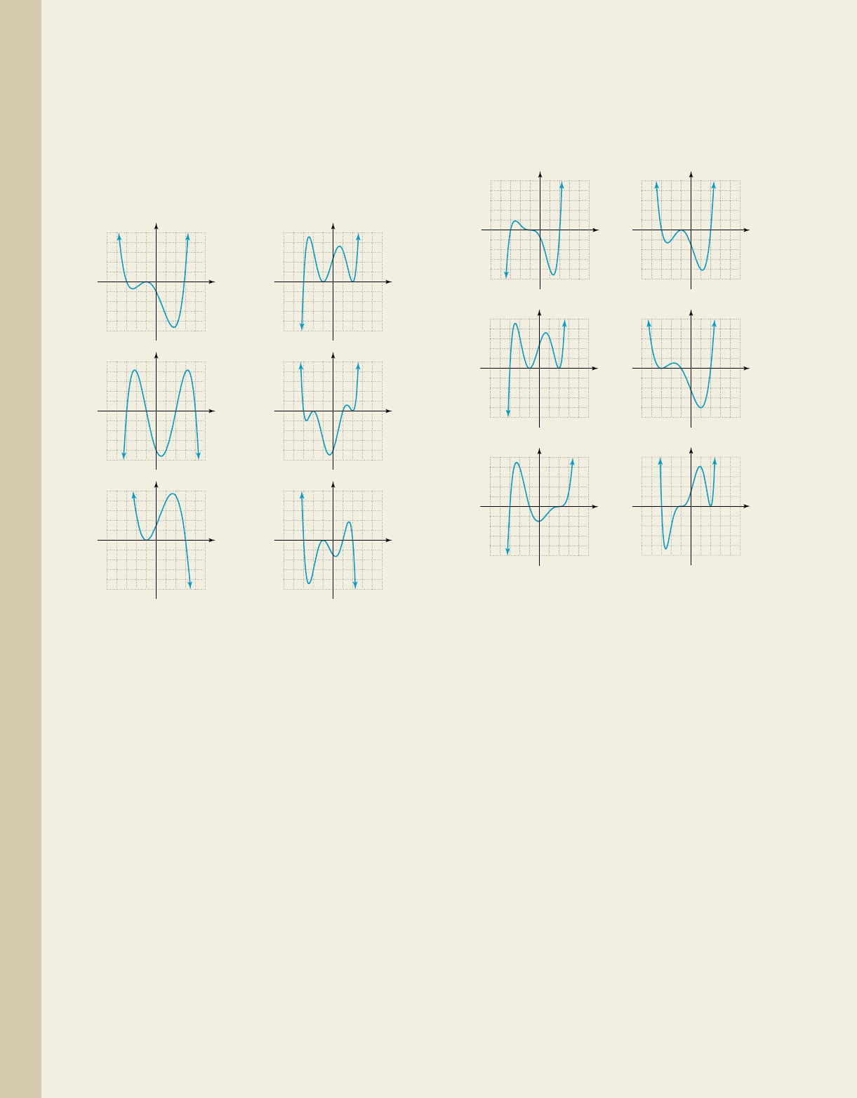
Determine whether each graph is the graph of a
polynomial function. If yes, state the least possible
degree of the function. If no, state why.
7. 8.
9. 10.
11. 12.
5432154321
1
2
3
4
5
2
3
4
5
1
x
y
f(x)
5432154321
1
2
3
4
5
2
3
4
5
1
x
y
q(x)
5432154 321
1
2
3
4
5
2
3
4
5
1
x
y
p(x)
5432154 321
1
2
3
4
5
2
3
4
5
1
x
y
g(x)
5432154321
1
2
3
4
5
2
3
4
5
1
x
y
h(x)
54321
5432
1
2
4
6
8
6
8
10
12
4
2
x
y
f(x)
State the end-behavior of the functions shown.
13. f(x) 14. g(x)
15. H(x) 16. h(x)
State the end-behavior and y-intercept of the functions
given. Do not graph.
17.
18.
19.
20.
21.
22. Y
2
x
6
4x
5
4x
3
16x 12
Y
1
3x
5
x
3
7x
2
6
q1x22x
3
18x
2
7x 3
p1x22x
4
x
3
7x
2
x 6
g1x2 x
4
4x
3
2x
2
16x 12
f
1x2 x
3
6x
2
5x 2
108642108642
65
130
195
260
325
130
195
260
325
65
x
y
h(x)
5432154321
6
12
18
24
30
12
18
24
30
6
x
y
H(x)
543215432
1
6
12
18
24
30
12
18
24
30
6
x
y
g(x)
5432154321
2
4
6
8
10
4
6
8
10
2
x
y
f(x)
3. The graphs of and
both at but the graph of is
than the graph of at this point.Y
1
Y
2
x 2,
Y
2
1x 22
4
Y
1
1x 22
2
5. In your own words, explain/discuss how to find the
degree and y-intercept of a function that is given in
factored form. Use
to illustrate.
f
1x2 1x 12
3
1x 221x 42
2
4. Since for all x, the ends of its graph will
always point in the direction. Since
when and when
the ends of its graph will always point in the
direction.
x 6 0,x
3
6 0x 7 0x
3
7 0
x
4
7 0
cob19545_ch04_411-429.qxd 11/26/10 7:44 AM Page 423
424 CHAPTER 4 Polynomial and Rational Functions 4–44
College Algebra Graphs & Models—
For each polynomial graph, (a) state whether the degree
of the function is even or odd; (b) use the graph to name
the zeroes of f, then state whether their multiplicity is
even or odd; (c) state the minimum possible degree of f
and write one possible function for f in factored form;
and (d) estimate the domain and range. Assume all
zeroes are real.
23. 24.
25. 26.
27. 28.
State the degree of each function, the end-behavior, and
y-intercept of its graph.
29.
30.
31.
32.
33.
34.
35.
36.
Every function in Exercises 37 through 42 has the zeroes
and . Match each to its
corresponding graph using degree, end-behavior, and
the multiplicity of each zero.
37.
38.
39. g1x2 1x 121x 321x 22
3
F1x2 1x 121x 32
2
1x 22
f
1x2 1x 12
2
1x 321x 22
x ⴝ 2x ⴝⴚ1, x ⴝⴚ3,
H1x2 1x 22
2
12 x21x
2
42
h1x2 1x
2
221x 12
2
11 x2
s1x2 1x 22
2
1x 12
2
1x
2
52
r1x2 1x
2
321x 42
3
1x 12
Y
2
1x 121x 22
3
15x 32
Y
1
1x 12
2
1x 2212x 321x 42
g1x2 1x 22
2
1x 421x 12
f
1x2 1x 321x 12
3
1x 22
2
5432154
3
21
4
8
12
16
20
8
12
16
20
4
x
y
5432154321
2
4
6
8
10
4
6
8
10
2
x
y
5432154321
12
24
36
48
60
24
36
48
60
12
x
y
5432154321
6
12
18
24
30
12
18
24
30
6
x
y
5432154321
2
4
6
8
10
4
6
8
10
2
x
y
54321
54321
2
4
6
8
10
4
6
8
10
2
x
y
40.
41.
42.
a. b.
c. d.
e. f.
Sketch the graph of each function using the degree, end-
behavior, x- and y-intercepts, zeroes of multiplicity, and
a few midinterval points to round-out the graph.
Connect all points with a smooth, continuous curve.
43.
44.
45.
46.
47.
48.
49.
50.
51.
52.
53.
54.
55.
56. Y
4
1x 321x 12
3
1x 12
2
Y
3
1x 12
3
1x 12
2
1x 22
H1x2 1x 321x 12
2
1x 22
2
h1x2 1x 12
3
1x 321x 22
g1x2 13x 421x 12
3
f 1x2 12x 321x 12
3
s1x21x 321x 12
2
1x 12
2
r1x21x 12
2
1x 22
2
1x 12
Y
2
1x 221x 12
2
15x 22
Y
1
1x 12
2
13x 221x 32
q1x21x 221x 22
2
p1x21x 12
2
1x 32
g1x2 1x 221x 421x 12
f
1x2 1x 321x 121x 22
5432154321
8
16
24
32
40
16
24
32
40
8
x
y
5432154321
16
32
48
64
80
32
48
64
80
16
x
y
5432154321
8
16
24
32
40
16
24
32
40
8
x
y
5432154321
5
10
15
20
25
10
15
20
25
5
x
y
5432154321
4
8
12
16
20
8
12
16
20
4
x
y
5432154321
8
16
24
32
40
16
24
32
8
x
40
y
Y
2
1x 12
3
1x 321x 22
2
Y
1
1x 12
2
1x 321x 22
2
G1x2 1x 12
3
1x 321x 22
cob19545_ch04_411-429.qxd 8/19/10 11:13 PM Page 424
4–45 Section 4.3 Graphing Polynomial Functions 425
College Algebra Graphs & Models—
Use the Guidelines for Graphing Polynomial Functions to
graph the polynomials.
57.
58.
59.
60.
61.
62.
63.
64.
65.
66.
67.
68.
69.
70.
71.
72.
73.
74. g1x2 x
5
3x
4
x
3
3x
2
f 1x2 x
5
4x
4
16x
2
16x
G1x2 3x
4
2x
3
8x
2
F1x2 2x
4
3x
3
9x
2
Y
4
2x
4
3x
3
15x
2
32x 12
Y
3
3x
4
2x
3
36x
2
24x 32
Y
2
x
4
4x
3
3x
2
10x 8
Y
1
x
4
6x
3
8x
2
6x 9
s1x2 x
4
5x
3
20x 16
r1x2 x
4
9x
2
4x 12
q1x2x
4
13x
2
36
p1x2x
4
10x
2
9
H1x2x
3
x
2
8x 12
h1x2x
3
x
2
5x 3
g1x2 x
3
2x
2
5x 6
f
1x2 x
3
3x
2
6x 8
y x
3
13x 12
y x
3
3x
2
4
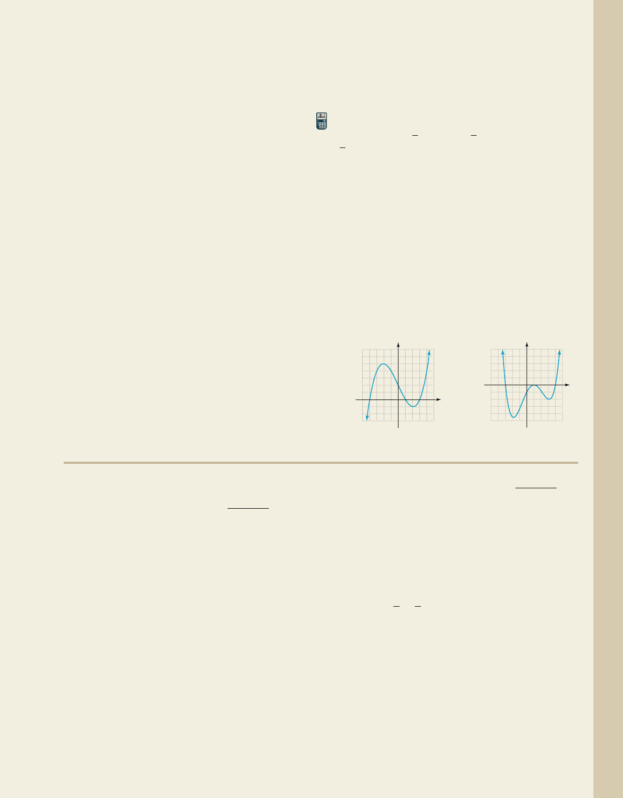
75.
76.
In preparation for future course work, it becomes
helpful to recognize the most common square roots
in mathematics: and
Graph the following polynomials on a
graphing calculator, and use the calculator to locate the
maximum/minimum values and all zeroes. Use the zeroes
to write the polynomial in factored form, then verify the
y-intercept from the factored form and polynomial form.
77.
78.
79.
80.
Use the graph of each function to construct its equation in
factored form and in polynomial form. Be sure to check
the y-intercept and adjust the lead coefficient if necessary.
81. 82.
5432154321
3
2
1
4
5
2
3
4
5
1
x
y
5432154321
1
2
3
4
5
6
7
3
2
1
x
y
g1x2 3x
5
2x
4
24x
3
16x
2
36x 24
f
1x2 2x
5
5x
4
10x
3
25x
2
12x 30
H1x2 x
5
5x
4
4x 20
h1x2 x
5
4x
4
9x 36
16 ⬇ 2.449.
12 ⬇ 1.414, 13 ⬇ 1.732,
H1x2 x
6
3x
5
4x
4
h1x2 x
6
2x
5
4x
4
8x
3
䊳
WORKING WITH FORMULAS
83. Roots tests for a quartic polynomial
:
In the Chapter 3 Reinforcing Basic Concepts
feature, we used relationships between the roots of
a quadratic equation and its coefficients to verify
the roots without having to substitute. Similar
root/coefficient relationships exist for cubic and
quartic polynomials, but the method soon becomes
too time consuming (see Exercise 94). There is
actually a little known formula for checking the
roots of a quartic polynomial (and others) that is
much more efficient. Given that r
1
, r
2
, r
3
, and r
4
are the roots of the polynomial, the sum of the
1r
1
2
2
ⴙ 1r
2
2
2
ⴙ 1r
3
2
2
ⴙ 1r
4
2
2
ⴝ
b
2
ⴚ 2ac
a
2
ax
4
ⴙ bx
3
ⴙ cx
2
ⴙ dx ⴙ e
squares of the roots must be equal to .
Note that if , the formula reduces to .
(a) Use this test to verify that , , 2, and 4
are the roots of ,
then (b) use these roots and the factored form to write
the equation in polynomial form to confirm results.
84. It is worth noting that the root test in Exercise 83
still applies when the roots are irrational and/or
complex. Use this test to verify that
and are the
solutions to then
use these zeroes and the factored form to write the
equation in polynomial form to confirm results.
x
4
2x
3
2x
2
6x 15 0,
1 2ix 13
, 13, 1 2i,
x
4
2x
3
13x
2
14x 24 0
1x 3
b
2
2ca 1
b
2
2ac
a
2
cob19545_ch04_411-429.qxd 8/19/10 11:14 PM Page 425
426 CHAPTER 4 Polynomial and Rational Functions 4–46
College Algebra Graphs & Models—
䊳
APPLICATIONS
85. Traffic volume: Between the hours of 6:00
A
.
M
.
and 6.00
P
.
M
., the volume of traffic at a busy
intersection can be modeled by the polynomial
where v(t)
represents the number of vehicles above/below
average, and t is number of hours past 6:00
A
.
M
.
(6:00
A
.
M
. (a) Use the remainder theorem to
find the volume of traffic during rush hour
(8:00
A
.
M
.), lunch time (12 noon), and the trip
home (5:00
P
.
M
.). (b) Use the rational zeroes
theorem to find the times when the volume of
traffic is at its average (c) Use this
information to graph v(t), then use the graph to
estimate the maximum and minimum flow of traffic
and the time at which each occurs.
86. Insect population: The population of a certain
insect varies dramatically with the weather, with
springlike temperatures causing a population
boom and extreme weather (summer heat and
winter cold) adversely affecting the population.
This phenomena can be modeled by the polynomial
where p(m)
represents the number of live insects (in hundreds
of thousands) in month m .
(a) Use the remainder theorem to find the
population of insects during the cool of spring
(March) and the fair weather of fall (October).
(b) Use the rational zeroes theorem to find the
times when the population of insects becomes
dormant (c) Use this information to
graph p(m), then use the graph to estimate the
maximum and minimum population of insects, and
the month at which each occurs.
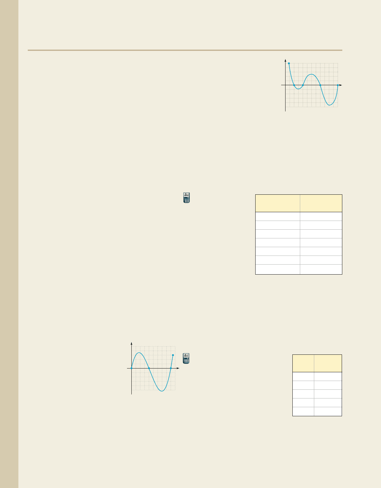
87. Balance of payments: The graph shown represents
the balance of payments (surplus versus deficit) for
a large county over a 9-yr period. Use it to answer
the following:
a. What is the minimum
possible degree
polynomial that can
model this graph?
b. How many years did this
county run a deficit?
c. Construct an equation
model in factored form and in polynomial
form, adjusting the lead coefficient as needed.
How large was the deficit in year 8?
88. Water supply: The graph shown represents the
water level in a reservoir (above and below normal)
that supplies water to a metropolitan area, over a
6-month period. Use it to answer the following:
3p1m2 04.
1m 僆 10, 14S Jan2
p1m2m
4
26m
3
217m
2
588m,
3v1t2 04.
S 02.
v1t2t
4
25t
3
192t
2
432t,
a. What is the
minimum possible
degree polynomial
that can model this
graph?
b. How many months
was the water level
below normal in this
6-month period?
c. At the beginning of this period the
water level was 36 in. above normal, due to a
long period of rain. Use this fact to help
construct an equation model in factored form
and in polynomial form, adjusting the lead
coefficient as needed. Use the equation to
determine the water level in months three
and five.
89. In order to
determine if the
number of lanes
on a certain
highway should
be increased, the
flow of traffic (in
vehicles per min)
is carefully
monitored from
6:00
A
.
M
. to
6:00
P
.
M
. The
data collected are shown the table (6:00
A
.
M
.
corresponds to ). (a) Draw a scatterplot and
decide on an appropriate form of regression, then
find the regression equation and graph the function
and scatterplot on the same screen. (b) Use the
regression equation and its graph to find the
maximum flow of traffic for the morning and
evening rush hours. (c) During what time(s) of day
is the flow rate 350 vehicles per hour?
90. The Goddard Memorial Rocket
Club is testing a new two-stage
rocket. Using a specialized
tracking device, the velocity of
the rocket is monitored every
second for the first 4.5 sec of
flight, with the data collected
in the table shown. (a) Draw a
scatterplot and decide on an
appropriate form of regression, then find the
regression equation and graph the function and
scatterplot on the same screen. (b) Use the
regression equation and its graph to find how many
seconds elapsed before the first stage burned out,
t 0
1m 02,
10987654321
6
4
2
8
10
4
6
8
10
2
Year
Balance
(10,000s)
(9.5, ~6)
Level
(inches)
Month
654321
6
4
2
8
10
4
6
8
10
2
Time Volume
(6:00
A
.
M
. ) (vehicles/min)
00
2 222
4 100
6 114
8 360
10 550
11 429
S 0
Time Velocity
(sec) (ft/sec)
00
1 441
2 484
3 459
4 696
cob19545_ch04_411-429.qxd 8/19/10 11:14 PM Page 426
4–47 Section 4.3 Graphing Polynomial Functions 427
College Algebra Graphs & Models—
and the rocket’s velocity at this time, then
(c) determine how many seconds elapsed (after
liftoff) until the second stage ignited. (d) At a
velocity of 1000 ft/sec, the fuel was exhausted and
the return chutes deployed. How many seconds
after liftoff did this occur?
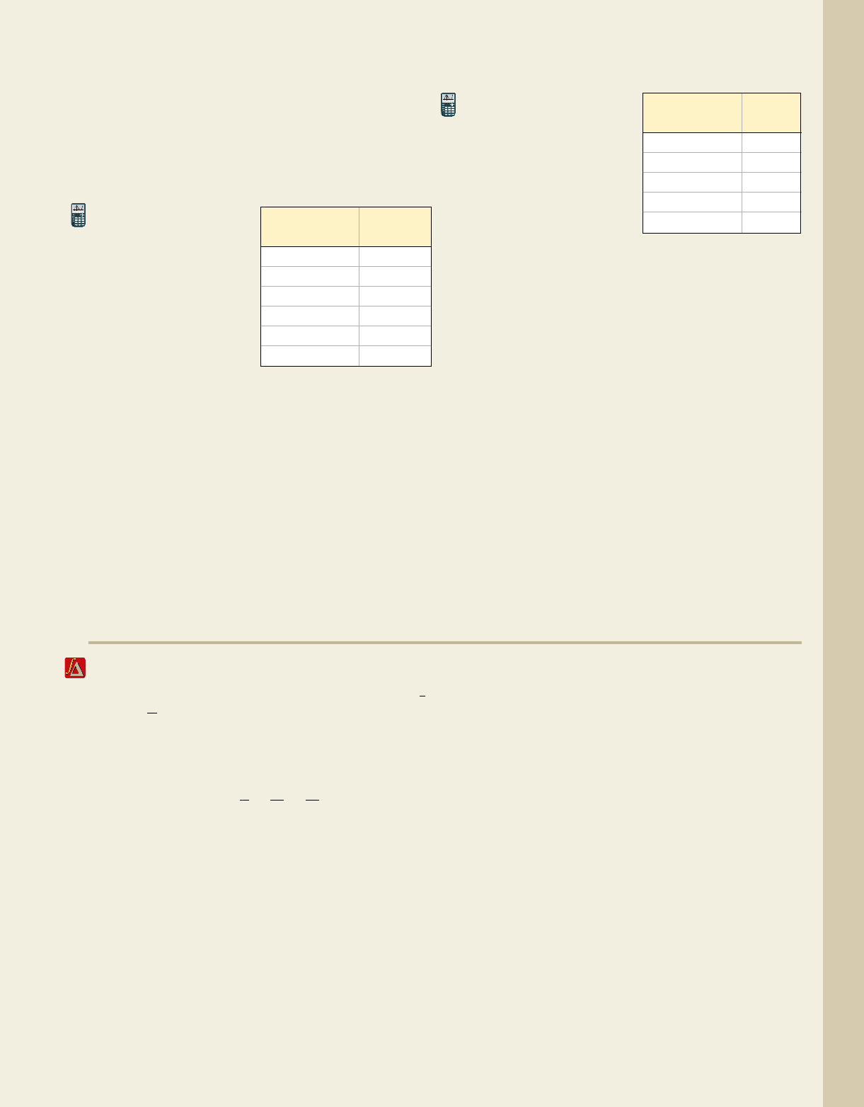
91. A posh restaurant
in a thriving
neighborhood opens
at 10
A
.
M
. for the
lunch crowd, and
closes at 9
P
.
M
. as the
dinner crowd leaves.
In order to ensure
that an adequate
number of cooks and
servers are available,
their hourly customer count is monitored each day
for 1 month with the data averaged and compiled in
the table shown. (a) Draw a scatterplot and decide
on an appropriate form of regression, then find the
regression equation and graph the function and
scatterplot on the same screen. (b) Use the
regression equation and its graph to find what time
the restaurant reaches its morning peak and its
evening peak. (c) At what time is business slowest,
and how many customers are in the restaurant at
that time? (d) Between what times is the restaurant
serving 100 customers or more?
92. Using the wind to
generate power is
becoming more and
more prevalent. While
most people are aware
that a wind turbine
generates more power
with a stronger wind,
many are not aware that
the generators are built with a stall mechanism to
protect the generator, blades, and infrastructure in
very high winds. This affects the actual power output
as the generator operates near its threshold. The
power output [in watts (W)] of a certain generator is
shown in the table for wind velocity v in miles per
hour. (a) Draw a scatterplot and decide on an
appropriate form of regression, then find the
regression equation and graph the function and
scatterplot on the same screen. (b) Use the regression
equation and its graph to find the maximum safe
power output for this generator, and the wind speed
at which this occurs. (c) What is the power output in
a 23 mph wind? (d) If the manufacturer stipulates
that the turbine will experience automatic shutdown
when power output exceeds 900 W, what is the
greatest wind speed this turbine can tolerate?
䊳
EXTENDING THE CONCEPT
93. As discussed in this section, the study of end-
behavior looks at what happens to the graph of a
function as Notice that as both
and approach zero. This fact can be used to
study the end-behavior of polynomial graphs.
a. For factoring out
gives the expression
What happens
to the value of the expression as
As ?
b. Factor out from
What happens to the value of the
expression as As How does
this affirm the end-behavior must be up/up?
x S q?x Sq?
5x 1.
g1x2 x
4
3x
3
4x
2
x
4
x S q
x Sq?
f
1x2 x
3
a1
1
x
3
x
2
6
x
3
b.
x
3
f 1x2 x
3
x
2
3x 6,
1
x
2
1
x
冟
x
冟
Sq,
冟
x
冟
Sq.
94. If u, v, w, and z represent the roots of the quartic
polynomial , then
the following relationships are true:
(a) (b)
(c)
and (d) . Use
these tests to verify that are the
solutions to
then use these zeroes and the factored form to write
the equation in polynomial form to confirm results.
95. For what value of c will three of the four real roots
of be shared by the
polynomial
Show the following equations have no rational roots.
96.
97. x
5
2x
4
x
3
2x
2
3x 4 0
x
5
x
4
x
3
x
2
2x 3 0
x
3
2x
2
5x 6 0?
x
4
5x
3
x
2
21x c 0
x
4
2x
3
13x
2
14x 24 0,
x 3, 1, 2, 4
u
#
v
#
w
#
z ev1uz wz2d,
u1vw wz2v1w z2 w1u z2 c,
u1v z2u v w z b,
ax
4
bx
3
cx
2
dx e 0
Time Customer
(10
A
.
M
. ) count
00
279
441
643
9 122
11 3
S 0
Wind velocity Power
(mph) (W)
20 419
25 623
30 635
35 593
40 639
cob19545_ch04_411-429.qxd 8/19/10 11:15 PM Page 427
428 CHAPTER 4 Polynomial and Rational Functions 4–48
College Algebra Graphs & Models—
䊳
MAINTAINING YOUR SKILLS
98. (3.6) Given and find the
compositions and
then state the domain of each.
99. (3.1) By direct substitution, verify that
is a solution to and name the
second solution.
100. (R.3/R.6) Solve each of the following equations.
a.
b.
c.
2
x 3
5
21
x
2
9
4
1x 1
3 12x 2
12x 52 16 x2 3 x 31x 22
x
2
2x 5 0
x 1 2i
1g ⴰ f 21x2,
H1x2h1x2 1f ⴰ g21x2
g1x2
1
x
,f 1x2 x
2
2x
101. (1.3) Determine if the relation shown is a function.
If not, explain how the definition of a function is
violated.
feline
canine
dromedary
equestrian
bovine
cow
horse
cat
camel
dog
MID-CHAPTER CHECK
1. Compute using
long division and write the result in two ways:
(a) and
(b) .
2. Given that is a factor of
use the rational zeroes theorem to
write f(x) in completely factored form.
3. Use the remainder theorem to evaluate given
4. Use the factor theorem to find a third-degree
polynomial having and as roots.
5. Use the intermediate value theorem to show that
has a root in the interval (2, 3).
6. Use the rational zeroes theorem, tests for and 1,
synthetic division, and the remainder theorem to
write in completely
factored form.
7. Find all the zeroes of h, real and complex:
8. Sketch the graph of p using its degree, end-behavior,
y-intercept, zeroes of multiplicity, and any
midinterval points needed, given
1x 121x 32.p1x2 1x 12
2
h1x2 x
4
3x
3
10x
2
6x 20.
f 1x2 x
4
5x
3
20x 16
1
g1x2 x
3
6x 4
x 1 ix 2
f
1x23x
4
7x
2
8x 11.
f
122,
8x
2
x 6,
f
1x2 2x
4
x
3
x 2
dividend
divisor
1quotient2
remainder
divisor
dividend 1quotient21divisor2 remainder
1x
3
8x
2
7x 142 1x 22
9. Use the Guidelines for Graphing to draw the graph
of
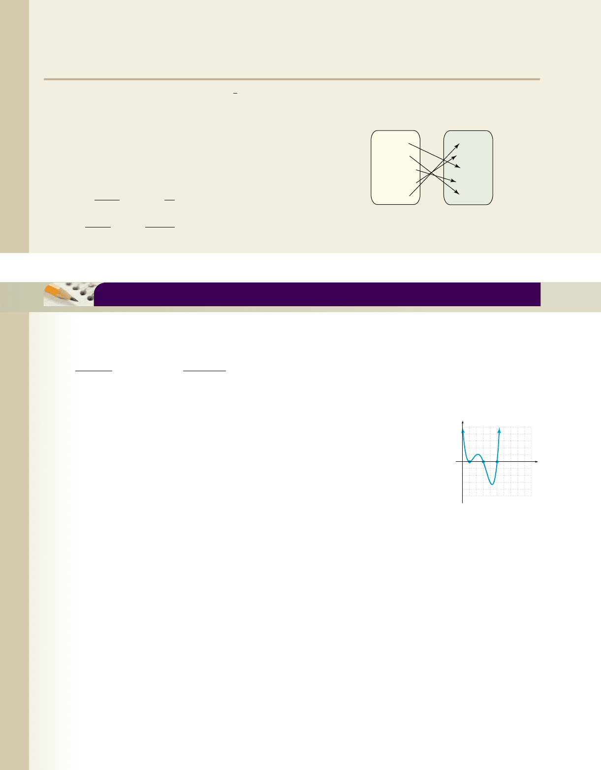
10. When fighter pilots train for dogfighting, a “hard-
deck” is usually established below which no
competitive activity can take place. The polynomial
graph given shows Maverick’s altitude above and
below this hard-deck during a 5-sec interval.
a. What is the minimum
possible degree
polynomial that could
form this graph? Why?
b. How many seconds
(total) was Maverick
below the hard-deck for
these 5 sec of the
exercise?
c. At the beginning of this time interval (t 0),
Maverick’s altitude was 1500 ft above the hard-
deck. Use this fact and the graph given to help
construct an equation model in factored form and
in polynomial form, adjusting the lead coefficient
if needed. Use the equation to determine
Maverick’s altitude in relation to the hard-deck at
and t 4.t 2
q1x2 x
3
5x
2
2x 8.
Altitude
(100s of feet)
10987612345
3
6
9
12
15
6
9
12
15
3
A
t
Seconds
cob19545_ch04_411-429.qxd 11/29/10 10:40 AM Page 428
4–49 Reinforcing Basic Concepts 429
College Algebra Graphs & Models—
REINFORCING BASIC CONCEPTS
Consider the equation Using the rational zeroes theorem, the possible rational zeroes are
The tests for 1 and indicate that neither is a zero: and Descartes’
rule of signs reveals there must be one positive real zero since the coefficients of change sign one time:
and one negative real zero since also changes sign one time:
The remaining two zeroes must be complex. Using with synthetic division shows 2 is not a
zero, but the coefficients in the quotient row are all positive, so 2 is an upper bound:
Using shows that is a zero and a lower bound for all other zeroes (quotient row alternates in sign):2x 2
coefficients of
f
(
x
)
q
(
x
)
2
|
110 16
2612 26
13613
|
20
x 2x
4
x
3
x 6.
f
1x2f 1x2f 1x2 x
4
x
3
x 6,
f
1x2
f
1127.f 1123151, 6, 2, 36.
x
4
x
3
x 6 0.
This means the remaining real zero must be a positive irrational
number less than 2 (all other possible rational zeroes were eliminated). The
quotient polynomial is not factorable, yet we’re
left with the challenge of finding this final zero. While there are many
advanced techniques available for approximating irrational zeroes, at this
level either technology or a technique called bisection is commonly used.
The bisection method combines the intermediate value theorem with
successively smaller intervals of the input variable, to narrow down the
location of the irrational zero. Although “bisection” implies halving the
interval each time, any number within the interval will do. The bisection
method may be most efficient using a succession of short input/output
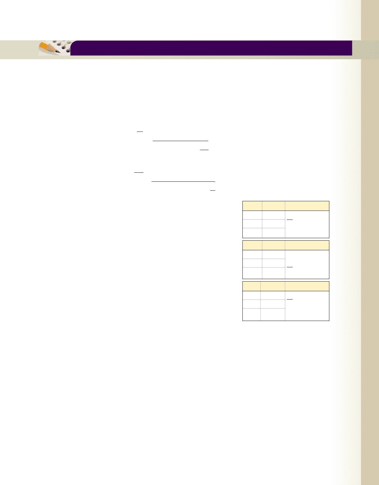
tables as shown, with the number of tables increased if greater accuracy is
desired. Since and the intermediate value theorem
tells us the zero must be in the interval [1, 2]. We begin our search here,
rounding noninteger outputs to the nearest 100th. As a visual aid, positive
outputs are in blue, negative outputs in red.
A reasonable estimate for the zero appears to be Evaluating
the function at this point gives which is very close
to zero. Naturally, a closer approximation is obtained using the capabilities of a graphing calculator. To seven decimal
places the zero is
Exercise 1: Use the intermediate value theorem to show that has a zero in the interval [1, 2], then
use bisection to locate the zero to three decimal place accuracy.
Exercise 2: The function has two real zeroes in the interval Use the intermediate value
theorem to locate the zeroes, then use bisection to find the zeroes accurate to three decimal places.
35, 54.f
1x2 x
4
3x 15
f
1x2 x
3
3x 1
x ⬇ 1.2756822.
f 11.2752⬇ 0.0097,
x 1.275.
f
122 20,f 1123
q
1
1x2 x
3
x
2
2x 3
coefficients of
f
(
x
)
q
1
(
x
)
2
|
11016
2246
1 123
|
0
xf(x) Conclusion
1
1.5 3.94
2 20
3
Zero is here,
use
next
x 1.25
xf(x) Conclusion
1
1.25
1.5 3.94
0.36
3
Zero is here,
use
next
x 1.30
xf(x) Conclusion
1.25
1.30
1.5 3.94
0.35
0.36
Zero is here,
use
next
x 1.275
Approximating Real Zeroes
—
—
—
cob19545_ch04_411-429.qxd 8/19/10 11:16 PM Page 429
